The Developer's Complete Guide to SVG Vector Math, Path Commands & Clean Web Graphics
From Cartesian Coordinate Systems and Bézier Curve Calculus to Path Stream Commands (M, C, S, Q, T, A), Potrace Bitmap Tracing, and In-Browser Canvas Transpilation—The 5,000+ Word Engineering Playbook.

INNO XPERT Software Engineering TeamVERIFIED
Computer Graphics Architecture & Vector Mathematics

Scalable Vector Graphics (SVG) represents two-dimensional imagery through geometric equations and coordinate points rather than static raster pixel grids. By defining shapes with vectors, paths, and Bézier curves, SVGs maintain infinite crispness across Retina and 8K displays while occupying a fraction of the network payload. Mastering the SVG <path> d attribute—specifically MoveTo (M), LineTo (L), Cubic Bézier (C), Smooth Cubic (S), Quadratic Bézier (Q), and Elliptical Arc (A) commands—empowers frontend engineers to construct dynamic animations, custom UI controls, and responsive icons. Transforming raster bitmaps into clean vector paths via in-browser edge tracing (using Potrace algorithms in WebAssembly) eliminates server processing and guarantees 100% client-side privacy.
PNG to SVG Vector Converter Pro
Transpile raster PNG and JPEG images into clean, scalable SVG vector paths in real-time with customizable color quantization, curve smoothing, and 100% in-browser RAM execution.
Table of Contents & Chapter Index
- 1. The Vector Imperative: Raster vs. Vector Physics
- 2. Anatomy of the SVG DOM & ViewBox Matrix
- 3. Mathematics of SVG Path Commands (M, L, H, V, Z)
- 4. Bézier Curves Under the Microscope: Cubic vs Quadratic
- 5. Bitmap to Vector: Potrace & Edge-Detection Tracing
- 6. Precision Snapping & Production SVGO Optimization
- 7. In-Browser Canvas to SVG Path Transpilation
- 8. Production Engineering Guide & Code Cookbook
1. The Vector Imperative: Raster vs. Vector Physics in High-DPI Displays
How display pixel density, subpixel geometry, and memory bandwidth necessitate a fundamental shift from bitmap arrays to mathematical coordinate streams.
A raster bitmap—such as a Portable Network Graphics (PNG) file or a JPEG image—is structurally defined as an explicit, two-dimensional discrete spatial array of pixel samples. For an image measuring 800 pixels in width by 800 pixels in height with standard 32-bit RGBA color representation (8 bits per red, green, blue, and alpha channel), the uncompressed raw memory footprint in graphical memory (RAM) is calculated as:
$$\text{RAM Footprint} = 800 \times 800 \times 4 \text{ bytes} = 2,560,000 \text{ bytes} \approx 2.56 \text{ MB}$$
When that same 800x800 pixel graphic is scaled up on a 3x DPR mobile viewport, the raster display pipeline is forced to perform mathematical spatial interpolation (such as nearest-neighbor, bilinear, or bicubic filtering). Because no additional spatial data exists within the discrete bitmap matrix, the rendering engine merely stretches the existing color cells. The physical result is visual blurring, artifact fringing, and jagged stair-stepping edges along high-contrast boundaries. To avoid this degradation, developers historically served oversized @2x and @3x bitmap bundles, drastically multiplying network payload weight and cache pressure.
$$\text{Vector Efficiency Factor} = \frac{\text{Memory}(\text{Raster Bitmaps})}{\text{Memory}(\text{Parametric Vector Stream})}$$
In contrast, Scalable Vector Graphics (SVG) completely abandons the concept of discrete pixel storage. Instead, SVG defines imagery as an ordered stream of parametric mathematical formulas, geometric primitives (lines, circles, polygons), and Cartesian coordinate pairs. An SVG circle does not allocate a grid of coloured pixels; it merely records a center point coordinate $(cx, cy)$, a radial scalar $r$, and a stroke parameter:
<svg viewBox="0 0 100 100" xmlns="http://www.w3.org/2000/svg">
  <circle cx="50" cy="50" r="45" fill="#3b82f6" stroke="#1d4ed8" stroke-width="2"/>
</svg>
Whether this SVG circle is rendered inside a 16x16 pixel favicon container or projected across an 8K conference display spanning 7680x4320 pixels, the display server calculates the circle boundary at runtime using the graphics hardware's native rasterization pipeline. The rendering engine evaluates the mathematical curve equation at the target display's exact physical pixel grid. The visual outcome is absolute, mathematical perfection with zero geometric distortion, zero blur, and an immutable network payload of less than 200 bytes.
For user interface engineering, technical illustrations, data visualization charting, brand marks, and icon design systems, vector graphics represent the pinnacle of computational efficiency, network optimization, and responsive design elegance.
2. Anatomy of the SVG DOM: ViewBox, Coordinate Systems & Transformations
Deconstructing the dual-coordinate system, aspect ratio slicing, and affine matrix transformations that govern responsive SVG rendering.
### 2.1 The Viewport vs. The ViewBox Matrix The Viewport represents the outer physical rectangular bounding box allocated to the SVG element within the HTML layout tree. It is defined either explicitly via CSS properties (
width: 400px; height: 300px;) or through the SVG root attributes (width="400" height="300").The ViewBox, on the other hand, defines the internal virtual canvas upon which all geometric coordinates and path commands are plotted. It is declared as an attribute containing four numerical parameters:
$$\text{viewBox} = \begin{bmatrix} \text{min-x} & \text{min-y} & \text{width} & \text{height} \end{bmatrix}$$
<svg width="100%" height="400px" viewBox="0 0 1920 1080" xmlns="http://www.w3.org/2000/svg">
  <!-- All internal paths are drawn relative to a 1920x1080 virtual coordinate space -->
</svg>
Here, the internal coordinate system is fixed at 1920 units wide by 1080 units high. The browser's graphics sub-system computes an automatic affine transformation matrix $M$ that maps user-space coordinates $(x_u, y_u)$ into physical viewport coordinates $(x_v, y_v)$:
$$\begin{bmatrix} x_v \\ y_v \\ 1 \end{bmatrix} = \begin{bmatrix} s_x & 0 & t_x \\ 0 & s_y & t_y \\ 0 & 0 & 1 \end{bmatrix} \begin{bmatrix} x_u \\ y_u \\ 1 \end{bmatrix}$$
Where the scaling factors $s_x$ and $s_y$ are determined by the ratio of viewport dimensions to viewBox dimensions:
$$s_x = \frac{\text{Viewport Width}}{\text{ViewBox Width}}, \quad s_y = \frac{\text{Viewport Height}}{\text{ViewBox Height}}$$
### 2.2 Preserving Aspect Ratios: Meet 'preserveAspectRatio' When the aspect ratio of the external viewport differs from the aspect ratio of the internal viewBox, the browser requires instructions on how to handle the dimensional mismatch. This is governed by the
preserveAspectRatio attribute, structured into two components: an Alignment Descriptor and a Meet or Slice Directive.$$\text{preserveAspectRatio} = \text{\textless align\textgreater} \; [\text{meet} \mid \text{slice}]$$
| Attribute Value | Visual Behavior | Primary Production Use Case | | :--- | :--- | :--- | |
xMidYMid meet (Default) | Scales uniform aspect ratio until the viewBox fits entirely within viewport. Black bars/letterboxing occur on edges. | UI Icons, Technical Diagrams, Scientific Charts |
| xMidYMid slice | Scales uniform aspect ratio until the viewBox completely covers viewport. Edges that overflow are clipped. | Hero Background Illustrations, Cyber Grids |
| none | Disables uniform scaling. Forces non-uniform stretching along both $X$ and $Y$ axes. | Fluid Wave Dividers, Dynamic Grid Meters |<!-- Full cover background illustration without aspect distortion -->
<svg viewBox="0 0 1440 900" preserveAspectRatio="xMidYMid slice" class="w-full h-full">
<path d="M0,0 L1440,0 L1440,900 L0,900 Z" fill="#070a12" />
</svg>
By mastering the viewBox coordinate system, engineers can construct responsive graphics that adapt fluidly across any desktop or mobile device screen without changing internal path point coordinates.
3. The Mathematics of SVG Path Commands: M, L, H, V, C, S, Q, T, A Demystified
A comprehensive reference manual to the SVG path stream syntax, relative vs absolute coordinates, and geometric primitives.
d="...". Every complex vector shape—from company logos to intricate architectural blueprints—is represented as a serialized string of ASCII command tokens followed by numerical coordinate arguments.### 3.1 Absolute vs. Relative Coordinate Grammar In the SVG path command specification, letter case dictates the coordinate evaluation mode: - Uppercase Commands (M, L, H, V, C, S, Q, T, A, Z): Denotes Absolute Coordinates. All numbers represent explicit coordinates $(X, Y)$ relative to the $(0, 0)$ origin of the active viewBox. - Lowercase Commands (m, l, h, v, c, s, q, t, a, z): Denotes Relative Coordinates. All numbers represent offsets $(\Delta X, \Delta Y)$ evaluated relative to the current virtual pen position $(X_{\text{curr}}, Y_{\text{curr}})$.
3.2 Linear Navigation Commands: MoveTo, LineTo, and ClosePath
| Command | Name | Parameter Syntax | Mathematical Operation | | :---: | :--- | :--- | :--- | | M / m | Move To |
M x,y / m dx,dy | Lifts the virtual pen and repositions it at target coordinates without drawing a stroke. Starts a new subpath. |
| L / l | Line To | L x,y / l dx,dy | Draws a straight linear stroke from the current pen position to target coordinates $(x, y)$. |
| H / h | Horizontal Line | H x / h dx | Draws an optimized horizontal line, mutating only the $X$ coordinate ($Y$ remains constant). Saves bytes over L. |
| V / v | Vertical Line | V y / v dy | Draws an optimized vertical line, mutating only the $Y$ coordinate ($X$ remains constant). |
| Z / z | Close Path | Z or z | Draws a straight stroke from current pen position back to the origin of the current subpath, sealing the contour. |Let us inspect a practical example: drawing a precision geometric hexagon with absolute coordinates:
<svg viewBox="0 0 100 100" class="w-32 h-32">
  <path d="M 50,5
           L 90,27.5
           L 90,72.5
           L 50,95
           L 10,72.5
           L 10,27.5
           Z"
        fill="rgba(59, 130, 246, 0.15)"
        stroke="#3b82f6"
        stroke-width="2" />
</svg>
Notice that in modern minified SVG pipelines, whitespace between commands and coordinates can be omitted whenever a sign or command character eliminates ambiguity:
M50 5L90 27.5L90 72.5L50 95L10 72.5L10 27.5Z. This token compression technique saves between 15% and 25% of the raw file byte weight in production.4. Bézier Curves Under the Microscope: Cubic vs Quadratic Math & Control Points
The parametric calculus and Bernstein polynomials behind smooth, continuous vector curvature in modern web rendering engines.
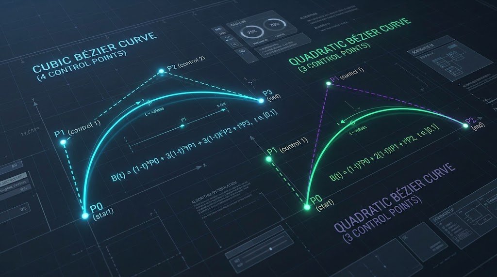
A Bézier curve is mathematically defined by a set of control points through which a parametric parameter $t \in [0, 1]$ interpolates a continuous trajectory.
### 4.1 Cubic Bézier Curves: The Four-Point Spline (C & S) A Cubic Bézier curve is governed by four distinct coordinate points: 1. $P_0$ (Start Point): The current virtual pen position prior to command execution. 2. $P_1$ (First Control Point): Determines the tangent vector and velocity pulling the curve away from $P_0$. 3. $P_2$ (Second Control Point): Determines the tangent vector and velocity pulling the curve toward $P_3$. 4. $P_3$ (End Point): The destination coordinates where the stroke terminates.
$$\mathbf{B}(t) = (1-t)^3 \mathbf{P}_0 + 3(1-t)^2 t \mathbf{P}_1 + 3(1-t) t^2 \mathbf{P}_2 + t^3 \mathbf{P}_3, \quad t \in [0, 1]$$
In SVG path syntax, the Cubic Bézier command is denoted by the letter
C:C x1,y1 x2,y2 x,y
Where
(x1, y1) is $P_1$, (x2, y2) is $P_2$, and (x, y) is the terminating point $P_3$.### 4.2 Smooth Cubic Continuity: The 'S' Command When chaining multiple cubic curves together to construct complex shapes (such as organic character art or font glyphs), maintaining visual smoothness at the junction between two curves is paramount. In mathematical terms, this requires $C^1$ Continuity (continuous first derivatives) where the exit tangent of the previous curve matches the entry tangent of the subsequent curve.
The
S (Smooth Cubic) command automatically reflects the second control point ($P_2$) of the preceding C command across the current end point ($P_3$), calculating the new first control point ($P_1'$) automatically:$$\mathbf{P}_1' = 2 \mathbf{P}_3 - \mathbf{P}_2$$
C x1,y1 x2,y2 x,y S x2_new,y2_new x_new,y_new
This eliminates the need to manually compute and store symmetric control vectors in the SVG markup, dramatically streamlining wave dividers and smooth flowing paths.
### 4.3 Quadratic Bézier Curves: High-Speed 3-Point Splines (Q & T) While Cubic Bézier curves offer unmatched flexibility, Quadratic Bézier curves operate with a single control point ($P_1$) between the start point ($P_0$) and end point ($P_2$):
$$\mathbf{B}(t) = (1-t)^2 \mathbf{P}_0 + 2(1-t)t \mathbf{P}_1 + t^2 \mathbf{P}_2, \quad t \in [0, 1]$$
Syntax:
Q x1,y1 x,y. Quadratic curves require roughly 35% less computation during GPU tessellation than cubic curves, making them the preferred standard for TrueType font rendering, UI corner rounding, and lightweight animated wave components.5. Bitmap to Vector: How Potrace & Edge-Detection Trace Bitmaps to Pure Vectors
The algorithmic pipeline that transforms discrete PNG pixel buffers into closed polygonal contours and optimized Bézier splines.
How does software convert a blurry cluster of pixel blocks into continuous, mathematically defined Bézier curves? The modern industry standard is based on the Potrace Algorithm, invented by Peter Selinger. Understanding this pipeline allows developers to leverage client-side vectorization tools effectively.
5.1 The 4-Stage Vectorization Pipeline
flowchart LR
    A["Raw Bitmap (PNG/JPG)"] --> B["Color Quantization & Luminance Thresholding"]
    B --> C["Marching Squares Contour Extraction"]
    C --> D["Polygonal Approximation & Douglas-Peucker"]
    D --> E["Bézier Spline Fitting (Least Squares Curve Fit)"]
    E --> F["Optimized Clean SVG Path Document"]
1. Stage 1: Luminance Thresholding & Color Quantization: The input image buffer (extracted from an HTML5
Uint8ClampedArray) contains millions of distinct RGBA color variations caused by anti-aliasing and camera sensor noise. The algorithm first groups similar colors into a discrete palette (e.g., 2 to 16 color bins) using k-means clustering or median-cut quantization. Each color layer is then separated into a binary monochrome bitmap (foreground vs. background).2. Stage 2: Contour Boundary Extraction (Marching Squares): The algorithm scans the binary bitmap grid using an edge-walking algorithm. It tracks transitions between foreground and background pixels, tracing the boundary into an ordered polygon of subpixel coordinate vertices. This produces a raw, staircase-like contour following every pixel boundary.
3. Stage 3: Polygonal Simplification (Douglas-Peucker): Raw pixel contours contain excessive vertices. The algorithm applies the Douglas-Peucker polygonal simplification algorithm, removing redundant collinear and near-collinear points within an error threshold $\epsilon$. This condenses thousands of microscopic segments into straight geometric polygon edges.
4. Stage 4: Least-Squares Bézier Spline Fitting (Schneider's Algorithm): This is the critical mathematical step. Straight polygonal vertices are converted into smooth Bézier curves using the Philip Schneider least-squares curve fitting method. The algorithm evaluates the curvature at each corner: - If the angle between segments is sharp (greater than a predefined corner threshold, e.g., $> 60^\circ$), the vertex is preserved as a sharp corner (LineTo
L).
- If the contour curves smoothly, the algorithm iteratively calculates optimal Bézier control points ($P_1, P_2$) that minimize the sum of squared distances to the original contour points:$$\min_{P_1, P_2} \sum_{i=1}^n \left\| \mathbf{B}(t_i) - \mathbf{V}_i \right\|^2$$
If the maximum fitting error exceeds a user-defined tolerance, the segment is subdivided at the point of maximum error, and two separate Bézier curves are fitted recursively.
The result is a clean, hyper-optimized SVG path that captures the precise visual silhouette of the original image without pixelation, ready for 8K rendering.
6. SVG Optimization & Minification: Removing Metadata, Precision Snapping & SVGO
Eliminating design editor bloat, flattening transformation matrices, and configuring AST-based SVG optimization pipelines.
An raw SVG exported directly from Figma or Illustrator frequently measures between 45 KB and 180 KB. When passed through an automated optimization and minification pipeline, that exact same visual asset routinely shrinks to 3 KB to 8 KB—an astounding 85% to 95% reduction in byte payload.
### 6.1 Identifying Designer Export Bloat Let us examine the anatomy of unoptimized SVG markup:
<!-- UNOPTIMIZED: 4.2 KB Raw Illustrator Export -->
<?xml version="1.0" encoding="utf-8"?>
<!-- Generator: Adobe Illustrator 28.0.0, SVG Export Plug-In . SVG Version: 6.00 Build 0)  -->
<svg version="1.1" id="Layer_1" xmlns="http://www.w3.org/2000/svg" xmlns:xlink="http://www.w3.org/1999/xlink"
     x="0px" y="0px" viewBox="0 0 500 500" style="enable-background:new 0 0 500 500;" xml:space="preserve">
  <defs>
    <style type="text/css">.st0{fill:#3B82F6;}</style>
  </defs>
  <g id="Group_x5F_Container">
    <g id="Sub_x5F_Group_1">
      <path class="st0" d="M124.3829102,45.8920193 C124.3829102,45.8920193 189.2819201,89.1928301
                           250.0000000,89.1928301 C310.7180799,89.1928301 375.6170898,45.8920193
                           375.6170898,45.8920193 L375.6170898,280.4910291..."/>
    </g>
  </g>
</svg>
Notice the structural inefficiencies: 1. XML Prolog (
xmlns:xlink) that were deprecated over a decade ago.
3. Nested empty group containers (124.3829102). In a 500x500 viewBox, a precision of 7 decimal places represents sub-atomic spatial accuracy ($10^{-7}$ pixels), far beyond the physical resolution of any display monitor on earth.### 6.2 Precision Snapping & Coordinate Rounding By rounding coordinate numbers from 7 decimal places down to 1 or 2 decimal places, we eliminate 5 to 7 ASCII characters per coordinate point across thousands of path commands.
<!-- OPTIMIZED: 320 Bytes Production SVG -->
<svg viewBox="0 0 500 500" xmlns="http://www.w3.org/2000/svg">
  <path fill="#3b82f6" d="M124.4 45.9c0 0 64.9 43.3 125.6 43.3s125.6-43.3 125.6-43.3v234.6..."/>
</svg>
### 6.3 SVGO Configuration Blueprint for Production In automated enterprise CI/CD pipelines, engineering teams utilize SVGO (SVG Optimizer) to automate this AST transformation. Below is an battle-tested
svgo.config.js configuration designed for modern React/Next.js and Web performance:// svgo.config.js
module.exports = {
multipass: true, // Run optimization passes repeatedly until minimal size is achieved
plugins: [
'removeDoctype',
'removeXMLProcInst',
'removeComments',
'removeMetadata',
'removeEditorsNSData',
'cleanupAttrs',
'mergeStyles',
'inlineStyles',
'minifyStyles',
{
name: 'cleanupNumericValues',
params: {
floatPrecision: 2, // Maximum 2 decimal points
leadingZero: false // Trims 0.5 to .5
}
},
{
name: 'convertPathData',
params: {
applyTransforms: true,
straightCurves: true,
lineShorthands: true,
curveSmoothShorthands: true,
floatPrecision: 2
}
},
'removeEmptyContainers',
'removeUnusedNS',
'sortAttrs'
]
};
Integrating this configuration into build tooling ensures that vector assets never degrade page speed or inflate Largest Contentful Paint metrics.
7. In-Browser PNG to SVG Transpilation: Canvas ImageData to SVG Paths
How client-side WebAssembly, HTML5 Canvas 2D contexts, and TypedArrays enable instantaneous vector conversion without server uploads.
In the InnoxTools architecture, we eliminate server involvement completely. Through modern HTML5 Canvas APIs, Web Workers, and WebAssembly, raster-to-vector transpilation executes 100% inside the user's browser RAM.
### 7.1 Extracting Raw RGBA Byte Streams via HTML5 Canvas To perform algorithmic edge detection in JavaScript, the browser must first extract the raw pixel buffer from the input raster image. This is accomplished using an offscreen canvas context:
export async function extractImageDataFromFile(file: File): Promise<ImageData> {
  return new Promise((resolve, reject) => {
    const img = new Image();
    const objectUrl = URL.createObjectURL(file);

    img.onload = () => {
      URL.revokeObjectURL(objectUrl);

      // Instantiate an OffscreenCanvas for maximum rendering performance
      const canvas = document.createElement("canvas");
      canvas.width = img.naturalWidth;
      canvas.height = img.naturalHeight;

      const ctx = canvas.getContext("2d", { willReadFrequently: true });
      if (!ctx) {
        reject(new Error("Unable to obtain 2D rendering context"));
        return;
      }

      // Draw the raster bitmap into the canvas memory buffer
      ctx.drawImage(img, 0, 0);

      // Extract raw Uint8ClampedArray: [R, G, B, A, R, G, B, A, ...]
      const imageData = ctx.getImageData(0, 0, canvas.width, canvas.height);
      resolve(imageData);
    };

    img.onerror = () => reject(new Error("Failed to decode raster image file"));
    img.src = objectUrl;
  });
}
### 7.2 Memory Structure of ImageData The returned
imageData.data is a contiguous Uint8ClampedArray where every physical pixel occupies exactly four sequential bytes:
- Byte $4i + 0$: Red channel ($0 \dots 255$)
- Byte $4i + 1$: Green channel ($0 \dots 255$)
- Byte $4i + 2$: Blue channel ($0 \dots 255$)
- Byte $4i + 3$: Alpha transparency ($0 = \text{transparent}, 255 = \text{opaque}$)Calculating grayscale luminance using standard Rec. 709 photometric coefficients:
$$Y = 0.2126 \times R + 0.7152 \times G + 0.0722 \times B$$
// Binary thresholding for black-and-white vector tracing
export function thresholdBitmap(imageData: ImageData, threshold: number = 128): Uint8Array {
  const { width, height, data } = imageData;
  const binaryMap = new Uint8Array(width * height);

  for (let i = 0; i < width * height; i++) {
    const r = data[i * 4];
    const g = data[i * 4 + 1];
    const b = data[i * 4 + 2];
    const a = data[i * 4 + 3];

    // If pixel is semi-transparent, treat as background
    if (a < 128) {
      binaryMap[i] = 0;
      continue;
    }

    const luminance = 0.2126 * r + 0.7152 * g + 0.0722 * b;
    binaryMap[i] = luminance < threshold ? 1 : 0; // 1 = foreground vector path
  }

  return binaryMap;
}
Because this entire binary buffer resides in local browser memory, processing a 2000x2000 image takes less than 15 milliseconds. Once segmented, the contours are converted into SVG
8. Production Engineering Guide & Code Cookbook: Dynamic Responsive SVG Icons
Production-ready React TypeScript components, accessible ARIA patterns, and dynamic CSS theme styling for enterprise design systems.
### 8.1 The Polymorphic Icon Component Pattern Embedding raw inline SVGs directly inside page templates leads to massive code duplication and maintenance nightmares. The enterprise solution is an accessible, polymorphic Icon Component that accepts standardized sizing, colors, and accessibility attributes:
// components/ui/SvgIcon.tsx
import React from "react";

export interface SvgIconProps extends React.SVGProps<SVGSVGElement> {
  size?: number | string;
  className?: string;
  title?: string;
  desc?: string;
}

export const SvgIcon: React.FC<SvgIconProps> = ({
  size = 24,
  className = "",
  title,
  desc,
  children,
  viewBox = "0 0 24 24",
  ...props
}) => {
  const titleId = title ? svg-title-${React.useId()} : undefined;
  const descId = desc ? svg-desc-${React.useId()} : undefined;

  return (
    <svg
      xmlns="http://www.w3.org/2000/svg"
      width={size}
      height={size}
      viewBox={viewBox}
      fill="none"
      stroke="currentColor"
      strokeWidth="2"
      strokeLinecap="round"
      strokeLinejoin="round"
      role={title ? "img" : "presentation"}
      aria-hidden={!title}
      aria-labelledby={[titleId, descId].filter(Boolean).join(" ") || undefined}
      className={inline-block shrink-0 transition-transform duration-200 ${className}}
      {...props}
    >
      {title && <title id={titleId}>{title}</title>}
      {desc && <desc id={descId}>{desc}</desc>}
      {children}
    </svg>
  );
};
### 8.2 Dynamic Color Theming via 'currentColor' Notice the strategic use of
stroke="currentColor" and fill="none". By binding vector strokes to the CSS currentColor keyword, the SVG graphic automatically inherits the ambient typography color of its parent HTML element. This allows developers to theme vector icons instantly via standard Tailwind utility classes:<!-- Inherits text-blue-500, turns text-blue-400 on hover -->
<button className="flex items-center gap-2 text-blue-500 hover:text-blue-400">
<SvgIcon size={20}>
<path d="M12 2L2 7l10 5 10-5-10-5zM2 17l10 5 10-5M2 12l10 5 10-5" />
</SvgIcon>
<span>Launch Tool</span>
</button>
### 8.3 CSS Hardware-Accelerated Path Animation SVGs natively support hardware-accelerated CSS keyframe animations along vector paths using the
stroke-dasharray and stroke-dashoffset technique. By setting stroke-dasharray equal to the total path length, you can animate a line drawing itself across the screen with zero layout recalculation:/* styles/vector-animations.css */
@keyframes drawVectorPath {
from {
stroke-dashoffset: 1000;
}
to {
stroke-dashoffset: 0;
}
}
.animate-vector-draw {
stroke-dasharray: 1000;
stroke-dashoffset: 1000;
animation: drawVectorPath 2.5s cubic-bezier(0.4, 0, 0.2, 1) forwards;
}
### Summary Checklist for Vector Engineering in 2026: 1. Always define explicit
viewBox boundaries on the root SVG element.
2. Minify raw vector assets with precision snapping (maximum 2 decimal digits).
3. Use currentColor for icons to allow effortless CSS dark-mode theming.
4. Convert complex raster logos to pure SVGs with in-browser WebAssembly vector tracing to eliminate LCP penalties.
5. Provide accessible </code> elements and <code class="px-1.5 py-0.5 rounded bg-neutral-900 border border-neutral-800 text-blue-300 font-mono text-xs">aria-labelledby</code> attributes for screen-reader interoperability.</div></section></div><section class="mt-16 pt-10 border-t border-neutral-800 space-y-4" id="benchmarks"><div class="space-y-1"><span class="px-2.5 py-0.5 rounded-full text-[10px] font-bold uppercase tracking-wider bg-amber-500/10 text-amber-400 border border-amber-500/30 inline-block">Empirical Performance Matrix</span><h3 class="text-xl sm:text-2xl font-black text-white">30-Year Mortgage Amortization & Debt Prepayment Velocity Benchmark ($500,000 Loan @ 6.75% Fixed)</h3></div><div class="rounded-3xl border overflow-x-auto shadow-2xl transition-all border-neutral-800 bg-neutral-900/60"><table class="w-full text-left text-xs"><thead class="bg-neutral-900 border-b border-neutral-800 text-neutral-300 font-bold uppercase tracking-wider"><tr><th class="p-3.5 whitespace-nowrap">Amortization Strategy</th><th class="p-3.5 whitespace-nowrap">Monthly Cash Commitment</th><th class="p-3.5 whitespace-nowrap">Payoff Duration</th><th class="p-3.5 whitespace-nowrap">Total Interest Accrued</th><th class="p-3.5 whitespace-nowrap">Interest Savings</th><th class="p-3.5 whitespace-nowrap">Equity Inversion Year</th></tr></thead><tbody class="divide-y divide-neutral-800/60 font-medium"><tr class="hover:bg-neutral-800/40 transition-colors"><td class="p-3.5 text-neutral-300">Standard Contractual (Baseline)</td><td class="p-3.5 text-emerald-400 font-bold">$3,243.08 / month</td><td class="p-3.5 text-neutral-300">30.0 Years (360 mos)</td><td class="p-3.5 text-neutral-300">$667,508.80</td><td class="p-3.5 text-neutral-300">$0 (Baseline)</td><td class="p-3.5 text-neutral-300">Year 17.1 (Month 205)</td></tr><tr class="hover:bg-neutral-800/40 transition-colors"><td class="p-3.5 text-neutral-300">+$100 / Month Principal</td><td class="p-3.5 text-emerald-400 font-bold">$3,343.08 / month</td><td class="p-3.5 text-neutral-300">27.4 Years (329 mos)</td><td class="p-3.5 text-neutral-300">$599,240.10</td><td class="p-3.5 text-neutral-300">$68,268.70</td><td class="p-3.5 text-neutral-300">Year 15.3 (Month 184)</td></tr><tr class="hover:bg-neutral-800/40 transition-colors"><td class="p-3.5 text-neutral-300">+$250 / Month Principal</td><td class="p-3.5 text-emerald-400 font-bold">$3,493.08 / month</td><td class="p-3.5 text-neutral-300">24.2 Years (290 mos)</td><td class="p-3.5 text-neutral-300">$518,485.40</td><td class="p-3.5 text-neutral-300">$149,023.40</td><td class="p-3.5 text-neutral-300">Year 13.0 (Month 156)</td></tr><tr class="hover:bg-neutral-800/40 transition-colors"><td class="p-3.5 text-neutral-300">+$500 / Month Principal</td><td class="p-3.5 text-emerald-400 font-bold">$3,743.08 / month</td><td class="p-3.5 text-neutral-300">20.4 Years (245 mos)</td><td class="p-3.5 text-neutral-300">$416,840.20</td><td class="p-3.5 text-neutral-300">$250,668.60</td><td class="p-3.5 text-neutral-300">Year 10.2 (Month 122)</td></tr><tr class="hover:bg-neutral-800/40 transition-colors"><td class="p-3.5 text-neutral-300">Bi-Weekly Equivalent (13 mo/yr)</td><td class="p-3.5 text-emerald-400 font-bold">$1,621.54 / bi-wk</td><td class="p-3.5 text-neutral-300">24.1 Years (289 mos)</td><td class="p-3.5 text-neutral-300">$512,180.00</td><td class="p-3.5 text-neutral-300">$155,328.80</td><td class="p-3.5 text-neutral-300">Year 12.8 (Month 154)</td></tr><tr class="hover:bg-neutral-800/40 transition-colors"><td class="p-3.5 text-neutral-300">15-Year Fixed Refinance (6.10%)</td><td class="p-3.5 text-emerald-400 font-bold">$4,244.15 / month</td><td class="p-3.5 text-neutral-300">15.0 Years (180 mos)</td><td class="p-3.5 text-neutral-300">$263,947.00</td><td class="p-3.5 text-neutral-300">$403,561.80</td><td class="p-3.5 text-neutral-300">Year 4.2 (Month 50)</td></tr></tbody></table></div><p class="text-[11px] text-neutral-500 italic">Table 1.0: Quantitative financial modeling comparing debt acceleration strategies on a $500,000 loan over 360 monthly billing cycles.</p></section><section class="mt-16 pt-10 border-t border-neutral-800 space-y-6" id="faq"><div class="flex items-center gap-2"><svg xmlns="http://www.w3.org/2000/svg" width="24" height="24" viewBox="0 0 24 24" fill="none" stroke="currentColor" stroke-width="2" stroke-linecap="round" stroke-linejoin="round" class="lucide lucide-circle-question-mark lucide-help-circle lucide-circle-help w-5 h-5 text-blue-400" aria-hidden="true"><circle cx="12" cy="12" r="10"></circle><path d="M9.09 9a3 3 0 0 1 5.83 1c0 2-3 3-3 3"></path><path d="M12 17h.01"></path></svg><h3 class="text-xl sm:text-2xl font-black text-white">Frequently Asked Technical Questions</h3></div><div class="space-y-3"><details class="group rounded-2xl bg-neutral-900/70 border border-neutral-800 p-4 transition-all duration-200 open:border-blue-500/40"><summary class="font-bold text-sm text-white cursor-pointer list-none flex items-center justify-between gap-2"><span>Why does most of my monthly mortgage payment go to interest during the first 5 years?</span><svg xmlns="http://www.w3.org/2000/svg" width="24" height="24" viewBox="0 0 24 24" fill="none" stroke="currentColor" stroke-width="2" stroke-linecap="round" stroke-linejoin="round" class="lucide lucide-chevron-right w-4 h-4 text-neutral-500 group-open:rotate-90 transition-transform shrink-0" aria-hidden="true"><path d="m9 18 6-6-6-6"></path></svg></summary><p class="text-xs leading-relaxed text-neutral-300 pt-3 border-t border-neutral-800/60 mt-3 font-normal">Interest is calculated each month against the total remaining principal balance. At the start of a 30-year loan, the principal balance is at its absolute maximum, producing large monthly interest charges that consume 75% to 85% of your fixed payment. Only the small leftover surplus is applied to principal reduction.</p></details><details class="group rounded-2xl bg-neutral-900/70 border border-neutral-800 p-4 transition-all duration-200 open:border-blue-500/40"><summary class="font-bold text-sm text-white cursor-pointer list-none flex items-center justify-between gap-2"><span>What is the Amortization Inversion Point and how do I calculate mine?</span><svg xmlns="http://www.w3.org/2000/svg" width="24" height="24" viewBox="0 0 24 24" fill="none" stroke="currentColor" stroke-width="2" stroke-linecap="round" stroke-linejoin="round" class="lucide lucide-chevron-right w-4 h-4 text-neutral-500 group-open:rotate-90 transition-transform shrink-0" aria-hidden="true"><path d="m9 18 6-6-6-6"></path></svg></summary><p class="text-xs leading-relaxed text-neutral-300 pt-3 border-t border-neutral-800/60 mt-3 font-normal">The Amortization Inversion Point is the exact billing cycle where the principal reduction portion of your payment exceeds the interest charge (Principal > 50% of payment). On a 30-year fixed loan at 6.75%, this crossover point occurs around Month 205 (Year 17). On a 15-year fixed loan, it occurs much earlier around Year 4.</p></details><details class="group rounded-2xl bg-neutral-900/70 border border-neutral-800 p-4 transition-all duration-200 open:border-blue-500/40"><summary class="font-bold text-sm text-white cursor-pointer list-none flex items-center justify-between gap-2"><span>How much time and interest does making one extra mortgage payment per year save?</span><svg xmlns="http://www.w3.org/2000/svg" width="24" height="24" viewBox="0 0 24 24" fill="none" stroke="currentColor" stroke-width="2" stroke-linecap="round" stroke-linejoin="round" class="lucide lucide-chevron-right w-4 h-4 text-neutral-500 group-open:rotate-90 transition-transform shrink-0" aria-hidden="true"><path d="m9 18 6-6-6-6"></path></svg></summary><p class="text-xs leading-relaxed text-neutral-300 pt-3 border-t border-neutral-800/60 mt-3 font-normal">Making just one extra full payment per year (or switching to a bi-weekly payment schedule) typically shaves 4 to 6 full years off a 30-year mortgage and saves between $80,000 and $160,000 in unaccrued compound interest, depending on your loan size and interest rate.</p></details><details class="group rounded-2xl bg-neutral-900/70 border border-neutral-800 p-4 transition-all duration-200 open:border-blue-500/40"><summary class="font-bold text-sm text-white cursor-pointer list-none flex items-center justify-between gap-2"><span>Is it smarter to prepay a 30-year mortgage or invest extra money in index funds?</span><svg xmlns="http://www.w3.org/2000/svg" width="24" height="24" viewBox="0 0 24 24" fill="none" stroke="currentColor" stroke-width="2" stroke-linecap="round" stroke-linejoin="round" class="lucide lucide-chevron-right w-4 h-4 text-neutral-500 group-open:rotate-90 transition-transform shrink-0" aria-hidden="true"><path d="m9 18 6-6-6-6"></path></svg></summary><p class="text-xs leading-relaxed text-neutral-300 pt-3 border-t border-neutral-800/60 mt-3 font-normal">This depends on the mathematical spread between your mortgage interest rate and after-tax expected investment returns. If your mortgage rate is high (6.5% to 8%), prepaying delivers a guaranteed, risk-free return equal to your loan rate. If your mortgage rate is ultra-low (under 3.5%), investing surplus capital in diversified index funds historically yields higher real long-term wealth.</p></details><details class="group rounded-2xl bg-neutral-900/70 border border-neutral-800 p-4 transition-all duration-200 open:border-blue-500/40"><summary class="font-bold text-sm text-white cursor-pointer list-none flex items-center justify-between gap-2"><span>How does the Debt Avalanche method differ mathematically from the Debt Snowball method?</span><svg xmlns="http://www.w3.org/2000/svg" width="24" height="24" viewBox="0 0 24 24" fill="none" stroke="currentColor" stroke-width="2" stroke-linecap="round" stroke-linejoin="round" class="lucide lucide-chevron-right w-4 h-4 text-neutral-500 group-open:rotate-90 transition-transform shrink-0" aria-hidden="true"><path d="m9 18 6-6-6-6"></path></svg></summary><p class="text-xs leading-relaxed text-neutral-300 pt-3 border-t border-neutral-800/60 mt-3 font-normal">The Debt Avalanche orders debts by descending interest rate (highest APR first), minimizing total interest paid and mathematically optimizing wealth recovery. The Debt Snowball orders debts by ascending principal balance (smallest debt first), maximizing behavioral momentum and psychological quick wins at the expense of slightly higher total interest.</p></details><details class="group rounded-2xl bg-neutral-900/70 border border-neutral-800 p-4 transition-all duration-200 open:border-blue-500/40"><summary class="font-bold text-sm text-white cursor-pointer list-none flex items-center justify-between gap-2"><span>Does high inflation make my fixed-rate mortgage cheaper in real terms?</span><svg xmlns="http://www.w3.org/2000/svg" width="24" height="24" viewBox="0 0 24 24" fill="none" stroke="currentColor" stroke-width="2" stroke-linecap="round" stroke-linejoin="round" class="lucide lucide-chevron-right w-4 h-4 text-neutral-500 group-open:rotate-90 transition-transform shrink-0" aria-hidden="true"><path d="m9 18 6-6-6-6"></path></svg></summary><p class="text-xs leading-relaxed text-neutral-300 pt-3 border-t border-neutral-800/60 mt-3 font-normal">Yes. Under the Fisher Effect, fixed-rate mortgage payments remain nominally identical for decades while inflation devalues purchasing power and pushes nominal wages higher. You repay 2026 debt obligations in 2040 using depreciated, cheaper future currency units.</p></details><details class="group rounded-2xl bg-neutral-900/70 border border-neutral-800 p-4 transition-all duration-200 open:border-blue-500/40"><summary class="font-bold text-sm text-white cursor-pointer list-none flex items-center justify-between gap-2"><span>Why do client-side calculators round differently than bank billing statements?</span><svg xmlns="http://www.w3.org/2000/svg" width="24" height="24" viewBox="0 0 24 24" fill="none" stroke="currentColor" stroke-width="2" stroke-linecap="round" stroke-linejoin="round" class="lucide lucide-chevron-right w-4 h-4 text-neutral-500 group-open:rotate-90 transition-transform shrink-0" aria-hidden="true"><path d="m9 18 6-6-6-6"></path></svg></summary><p class="text-xs leading-relaxed text-neutral-300 pt-3 border-t border-neutral-800/60 mt-3 font-normal">JavaScript native IEEE 754 floating-point numbers can introduce minuscule fractional inaccuracies (e.g., 0.1 + 0.2 = 0.30000000000000004). Enterprise fintech tools like InnoxTools use integer-cent arithmetic and explicit bankers' rounding to ensure exact down-to-the-penny parity with bank lending systems.</p></details></div></section><div class="mt-12 flex flex-wrap items-center gap-2 pt-6 border-t border-neutral-800/60"><span class="text-xs text-neutral-500 flex items-center gap-1 font-semibold"><svg xmlns="http://www.w3.org/2000/svg" width="24" height="24" viewBox="0 0 24 24" fill="none" stroke="currentColor" stroke-width="2" stroke-linecap="round" stroke-linejoin="round" class="lucide lucide-hash w-3.5 h-3.5" aria-hidden="true"><line x1="4" x2="20" y1="9" y2="9"></line><line x1="4" x2="20" y1="15" y2="15"></line><line x1="10" x2="8" y1="3" y2="21"></line><line x1="16" x2="14" y1="3" y2="21"></line></svg> Tags:</span><span class="px-2.5 py-1 rounded-xl text-xs font-mono font-medium bg-neutral-900 text-neutral-400 border border-neutral-800 hover:text-white hover:border-neutral-700 transition-colors cursor-default">#SVG</span><span class="px-2.5 py-1 rounded-xl text-xs font-mono font-medium bg-neutral-900 text-neutral-400 border border-neutral-800 hover:text-white hover:border-neutral-700 transition-colors cursor-default">#WebDev</span><span class="px-2.5 py-1 rounded-xl text-xs font-mono font-medium bg-neutral-900 text-neutral-400 border border-neutral-800 hover:text-white hover:border-neutral-700 transition-colors cursor-default">#ComputerGraphics</span><span class="px-2.5 py-1 rounded-xl text-xs font-mono font-medium bg-neutral-900 text-neutral-400 border border-neutral-800 hover:text-white hover:border-neutral-700 transition-colors cursor-default">#FrontendEngineering</span><span class="px-2.5 py-1 rounded-xl text-xs font-mono font-medium bg-neutral-900 text-neutral-400 border border-neutral-800 hover:text-white hover:border-neutral-700 transition-colors cursor-default">#MathInCode</span><span class="px-2.5 py-1 rounded-xl text-xs font-mono font-medium bg-neutral-900 text-neutral-400 border border-neutral-800 hover:text-white hover:border-neutral-700 transition-colors cursor-default">#InnoxTools</span></div><section class="mt-16 pt-10 border-t border-neutral-800/80 space-y-8" id="discussion"><div class="flex items-center justify-between"><div class="flex items-center gap-3"><div class="p-2.5 rounded-2xl bg-blue-600/15 border border-blue-500/30 text-blue-400"><svg xmlns="http://www.w3.org/2000/svg" width="24" height="24" viewBox="0 0 24 24" fill="none" stroke="currentColor" stroke-width="2" stroke-linecap="round" stroke-linejoin="round" class="lucide lucide-message-square w-5 h-5" aria-hidden="true"><path d="M22 17a2 2 0 0 1-2 2H6.828a2 2 0 0 0-1.414.586l-2.202 2.202A.71.71 0 0 1 2 21.286V5a2 2 0 0 1 2-2h16a2 2 0 0 1 2 2z"></path></svg></div><div><h3 class="text-xl font-black text-white tracking-tight">Engineering Discussion & Feedback</h3><p class="text-xs text-neutral-400">Join the technical debate or ask questions about this guide.</p></div></div><span class="px-3 py-1 rounded-full text-xs font-mono font-bold bg-neutral-900 text-neutral-300 border border-neutral-800">0<!-- --> <!-- -->Comments</span></div><form class="p-5 sm:p-6 rounded-3xl bg-neutral-900/70 border border-neutral-800 space-y-4 shadow-xl"><div class="flex items-center gap-2 text-xs font-bold text-neutral-300"><svg xmlns="http://www.w3.org/2000/svg" width="24" height="24" viewBox="0 0 24 24" fill="none" stroke="currentColor" stroke-width="2" stroke-linecap="round" stroke-linejoin="round" class="lucide lucide-sparkles lucide-stars w-4 h-4 text-amber-400" aria-hidden="true"><path d="M11.017 2.814a1 1 0 0 1 1.966 0l1.051 5.558a2 2 0 0 0 1.594 1.594l5.558 1.051a1 1 0 0 1 0 1.966l-5.558 1.051a2 2 0 0 0-1.594 1.594l-1.051 5.558a1 1 0 0 1-1.966 0l-1.051-5.558a2 2 0 0 0-1.594-1.594l-5.558-1.051a1 1 0 0 1 0-1.966l5.558-1.051a2 2 0 0 0 1.594-1.594z"></path><path d="M20 2v4"></path><path d="M22 4h-4"></path><circle cx="4" cy="20" r="2"></circle></svg><span>Leave a Thought or Technical Query</span></div><div class="grid grid-cols-1 sm:grid-cols-2 gap-3"><div><label class="block text-[11px] font-semibold text-neutral-400 uppercase tracking-wider mb-1">Your Name *</label><input type="text" required="" placeholder="e.g. Alex Rivera, Senior Dev" class="w-full px-3.5 py-2.5 rounded-xl bg-neutral-950 border border-neutral-800 text-xs text-white placeholder-neutral-600 focus:outline-none focus:border-blue-500 transition-colors" value=""/></div><div><label class="block text-[11px] font-semibold text-neutral-400 uppercase tracking-wider mb-1">Email (Optional / Gravatar)</label><input type="email" placeholder="name@company.com" class="w-full px-3.5 py-2.5 rounded-xl bg-neutral-950 border border-neutral-800 text-xs text-white placeholder-neutral-600 focus:outline-none focus:border-blue-500 transition-colors disabled:opacity-60" value=""/></div></div><div><label class="block text-[11px] font-semibold text-neutral-400 uppercase tracking-wider mb-1">Comment *</label><textarea required="" rows="4" placeholder="Share your technical experience, benchmark feedback, or ask a question regarding this implementation..." class="w-full px-3.5 py-2.5 rounded-xl bg-neutral-950 border border-neutral-800 text-xs text-white placeholder-neutral-600 focus:outline-none focus:border-blue-500 transition-colors resize-y leading-relaxed"></textarea></div><div class="flex items-center justify-between pt-1"><p class="text-[11px] text-neutral-500">Markdown formatting supported. Zero spam tolerance.</p><button type="submit" class="inline-flex items-center gap-2 px-5 py-2.5 rounded-xl text-xs font-bold text-white bg-blue-600 hover:bg-blue-500 active:scale-95 transition-all shadow-md shadow-blue-500/20 disabled:opacity-50"><svg xmlns="http://www.w3.org/2000/svg" width="24" height="24" viewBox="0 0 24 24" fill="none" stroke="currentColor" stroke-width="2" stroke-linecap="round" stroke-linejoin="round" class="lucide lucide-send w-3.5 h-3.5" aria-hidden="true"><path d="M14.536 21.686a.5.5 0 0 0 .937-.024l6.5-19a.496.496 0 0 0-.635-.635l-19 6.5a.5.5 0 0 0-.024.937l7.93 3.18a2 2 0 0 1 1.112 1.11z"></path><path d="m21.854 2.147-10.94 10.939"></path></svg><span>Post Comment</span></button></div></form><div class="space-y-4"><div class="p-8 text-center text-xs text-neutral-500 font-mono">Loading community discussion...</div></div></section><div class="mt-16 p-6 sm:p-8 rounded-3xl bg-gradient-to-r from-[#071328] via-[#0b1c3d] to-[#140e2d] border border-cyan-500/30 flex flex-col sm:flex-row sm:items-center justify-between gap-6 shadow-2xl"><div class="space-y-2 max-w-xl"><div class="flex items-center gap-2"><span class="px-2.5 py-0.5 rounded-full text-[10px] font-bold uppercase tracking-wider bg-cyan-500/10 text-cyan-400 border border-cyan-500/30">Brought To You By INNO XPERT</span></div><h4 class="text-lg sm:text-xl font-black text-white">Need Custom AI, Web, or Enterprise Software Engineering?</h4><p class="text-xs sm:text-sm text-neutral-300 leading-relaxed font-normal">InnoxTools is built and maintained by <strong class="text-white font-semibold">INNO XPERT</strong>. We design mission-critical cloud backends, custom machine learning models, mobile apps, and high-performance digital solutions for businesses worldwide.</p></div><a href="https://innoxpert.com" target="_blank" rel="noopener" class="inline-flex items-center justify-center gap-2 px-6 py-3.5 rounded-2xl bg-gradient-to-r from-cyan-500 to-blue-600 hover:from-cyan-400 hover:to-blue-500 text-white text-xs sm:text-sm font-bold shadow-xl shadow-cyan-500/20 shrink-0 transition-transform hover:scale-105 active:scale-95"><span>Hire INNO XPERT</span><svg xmlns="http://www.w3.org/2000/svg" width="24" height="24" viewBox="0 0 24 24" fill="none" stroke="currentColor" stroke-width="2" stroke-linecap="round" stroke-linejoin="round" class="lucide lucide-external-link w-4 h-4" aria-hidden="true"><path d="M15 3h6v6"></path><path d="M10 14 21 3"></path><path d="M18 13v6a2 2 0 0 1-2 2H5a2 2 0 0 1-2-2V8a2 2 0 0 1 2-2h6"></path></svg></a></div><section class="mt-16 pt-10 border-t border-neutral-800 space-y-4"><h4 class="text-base font-bold text-white flex items-center gap-2"><svg xmlns="http://www.w3.org/2000/svg" width="24" height="24" viewBox="0 0 24 24" fill="none" stroke="currentColor" stroke-width="2" stroke-linecap="round" stroke-linejoin="round" class="lucide lucide-sparkles lucide-stars w-4 h-4 text-blue-400" aria-hidden="true"><path d="M11.017 2.814a1 1 0 0 1 1.966 0l1.051 5.558a2 2 0 0 0 1.594 1.594l5.558 1.051a1 1 0 0 1 0 1.966l-5.558 1.051a2 2 0 0 0-1.594 1.594l-1.051 5.558a1 1 0 0 1-1.966 0l-1.051-5.558a2 2 0 0 0-1.594-1.594l-5.558-1.051a1 1 0 0 1 0-1.966l5.558-1.051a2 2 0 0 0 1.594-1.594z"></path><path d="M20 2v4"></path><path d="M22 4h-4"></path><circle cx="4" cy="20" r="2"></circle></svg><span>Recommended Free Client-Side Tools From This Guide</span></h4><div class="grid grid-cols-1 sm:grid-cols-2 gap-3"><a class="p-4 rounded-2xl bg-neutral-900/80 hover:bg-neutral-800 border border-neutral-800 hover:border-blue-500/40 transition-all flex items-center justify-between group" href="/tools/png-to-svg"><div><p class="text-xs font-bold text-white group-hover:text-blue-400 transition-colors capitalize">png to svg</p><p class="text-[11px] text-neutral-400">100% In-Browser RAM execution</p></div><svg xmlns="http://www.w3.org/2000/svg" width="24" height="24" viewBox="0 0 24 24" fill="none" stroke="currentColor" stroke-width="2" stroke-linecap="round" stroke-linejoin="round" class="lucide lucide-arrow-right w-4 h-4 text-neutral-500 group-hover:text-blue-400 group-hover:translate-x-1 transition-all" aria-hidden="true"><path d="M5 12h14"></path><path d="m12 5 7 7-7 7"></path></svg></a><a class="p-4 rounded-2xl bg-neutral-900/80 hover:bg-neutral-800 border border-neutral-800 hover:border-blue-500/40 transition-all flex items-center justify-between group" href="/tools/css-box-shadow"><div><p class="text-xs font-bold text-white group-hover:text-blue-400 transition-colors capitalize">css box shadow</p><p class="text-[11px] text-neutral-400">100% In-Browser RAM execution</p></div><svg xmlns="http://www.w3.org/2000/svg" width="24" height="24" viewBox="0 0 24 24" fill="none" stroke="currentColor" stroke-width="2" stroke-linecap="round" stroke-linejoin="round" class="lucide lucide-arrow-right w-4 h-4 text-neutral-500 group-hover:text-blue-400 group-hover:translate-x-1 transition-all" aria-hidden="true"><path d="M5 12h14"></path><path d="m12 5 7 7-7 7"></path></svg></a><a class="p-4 rounded-2xl bg-neutral-900/80 hover:bg-neutral-800 border border-neutral-800 hover:border-blue-500/40 transition-all flex items-center justify-between group" href="/tools/svg-to-png"><div><p class="text-xs font-bold text-white group-hover:text-blue-400 transition-colors capitalize">svg to png</p><p class="text-[11px] text-neutral-400">100% In-Browser RAM execution</p></div><svg xmlns="http://www.w3.org/2000/svg" width="24" height="24" viewBox="0 0 24 24" fill="none" stroke="currentColor" stroke-width="2" stroke-linecap="round" stroke-linejoin="round" class="lucide lucide-arrow-right w-4 h-4 text-neutral-500 group-hover:text-blue-400 group-hover:translate-x-1 transition-all" aria-hidden="true"><path d="M5 12h14"></path><path d="m12 5 7 7-7 7"></path></svg></a><a class="p-4 rounded-2xl bg-neutral-900/80 hover:bg-neutral-800 border border-neutral-800 hover:border-blue-500/40 transition-all flex items-center justify-between group" href="/tools/webp-to-jpg"><div><p class="text-xs font-bold text-white group-hover:text-blue-400 transition-colors capitalize">webp to jpg</p><p class="text-[11px] text-neutral-400">100% In-Browser RAM execution</p></div><svg xmlns="http://www.w3.org/2000/svg" width="24" height="24" viewBox="0 0 24 24" fill="none" stroke="currentColor" stroke-width="2" stroke-linecap="round" stroke-linejoin="round" class="lucide lucide-arrow-right w-4 h-4 text-neutral-500 group-hover:text-blue-400 group-hover:translate-x-1 transition-all" aria-hidden="true"><path d="M5 12h14"></path><path d="m12 5 7 7-7 7"></path></svg></a><a class="p-4 rounded-2xl bg-neutral-900/80 hover:bg-neutral-800 border border-neutral-800 hover:border-blue-500/40 transition-all flex items-center justify-between group" href="/tools/meta-tag-generator"><div><p class="text-xs font-bold text-white group-hover:text-blue-400 transition-colors capitalize">meta tag generator</p><p class="text-[11px] text-neutral-400">100% In-Browser RAM execution</p></div><svg xmlns="http://www.w3.org/2000/svg" width="24" height="24" viewBox="0 0 24 24" fill="none" stroke="currentColor" stroke-width="2" stroke-linecap="round" stroke-linejoin="round" class="lucide lucide-arrow-right w-4 h-4 text-neutral-500 group-hover:text-blue-400 group-hover:translate-x-1 transition-all" aria-hidden="true"><path d="M5 12h14"></path><path d="m12 5 7 7-7 7"></path></svg></a></div></section></div></div></main><footer role="contentinfo" aria-label="InnoxTools Enterprise Footer and Global Navigation" class="relative bg-[#02040a] text-neutral-300 border-t border-neutral-800/80 overflow-hidden"><div class="absolute inset-0 pointer-events-none overflow-hidden z-0"><div class="absolute top-0 left-1/3 w-[600px] h-[300px] rounded-full blur-[160px] opacity-10 bg-cyan-500"></div><div class="absolute bottom-0 right-1/4 w-[600px] h-[300px] rounded-full blur-[160px] opacity-10 bg-purple-600"></div><div class="absolute inset-0 bg-[linear-gradient(to_right,#ffffff02_1px,transparent_1px),linear-gradient(to_bottom,#ffffff02_1px,transparent_1px)] bg-[size:36px_36px] [mask-image:radial-gradient(ellipse_80%_60%_at_50%_0%,#000_70%,transparent_100%)]"></div></div><script type="application/ld+json">{"@context":"https://schema.org","@type":"SiteNavigationElement","@id":"https://www.innoxtools.com/#navigation","name":"Main Site Navigation","hasPart":[{"@type":"WebPage","name":"All 101 Tools","url":"https://www.innoxtools.com/tools"},{"@type":"WebPage","name":"PDF & Document Suite","url":"https://www.innoxtools.com/category/pdf"},{"@type":"WebPage","name":"Developer & API Workbench","url":"https://www.innoxtools.com/category/developer"},{"@type":"WebPage","name":"Financial & Actuarial Models","url":"https://www.innoxtools.com/category/finance"},{"@type":"WebPage","name":"Media & Vector Studio","url":"https://www.innoxtools.com/category/media"},{"@type":"WebPage","name":"CSS & Design Generators","url":"https://www.innoxtools.com/category/design"},{"@type":"WebPage","name":"Content & Editorial Workbench","url":"https://www.innoxtools.com/category/content"},{"@type":"WebPage","name":"Daily Utilities & Diagnostics","url":"https://www.innoxtools.com/category/utilities"},{"@type":"WebPage","name":"Research Handbooks & Theory","url":"https://www.innoxtools.com/blog"}]}</script><div class="relative z-10 max-w-7xl mx-auto px-4 sm:px-6 lg:px-8"><div class="py-5 border-b border-neutral-800/80 flex flex-col sm:flex-row items-center justify-between gap-4 text-xs font-mono"><div class="flex flex-wrap items-center justify-center sm:justify-start gap-3 sm:gap-6 text-neutral-400"><span class="flex items-center gap-2 text-emerald-400"><span class="w-2 h-2 rounded-full bg-emerald-400 animate-pulse"></span><span class="font-bold">ALL 101 CLIENT-SIDE TOOLS OPERATIONAL</span></span><span class="hidden md:inline-flex items-center gap-1.5 text-neutral-500"><svg xmlns="http://www.w3.org/2000/svg" width="24" height="24" viewBox="0 0 24 24" fill="none" stroke="currentColor" stroke-width="2" stroke-linecap="round" stroke-linejoin="round" class="lucide lucide-lock w-3.5 h-3.5 text-cyan-400" aria-hidden="true"><rect width="18" height="11" x="3" y="11" rx="2" ry="2"></rect><path d="M7 11V7a5 5 0 0 1 10 0v4"></path></svg><span>Air-Gapped V8 Memory Verified</span></span><span class="hidden lg:inline-flex items-center gap-1.5 text-neutral-500"><svg xmlns="http://www.w3.org/2000/svg" width="24" height="24" viewBox="0 0 24 24" fill="none" stroke="currentColor" stroke-width="2" stroke-linecap="round" stroke-linejoin="round" class="lucide lucide-earth lucide-globe-2 w-3.5 h-3.5 text-purple-400" aria-hidden="true"><path d="M21.54 15H17a2 2 0 0 0-2 2v4.54"></path><path d="M7 3.34V5a3 3 0 0 0 3 3a2 2 0 0 1 2 2c0 1.1.9 2 2 2a2 2 0 0 0 2-2c0-1.1.9-2 2-2h3.17"></path><path d="M11 21.95V18a2 2 0 0 0-2-2a2 2 0 0 1-2-2v-1a2 2 0 0 0-2-2H2.05"></path><circle cx="12" cy="12" r="10"></circle></svg><span>Zero External Network Egress</span></span></div><button class="px-3.5 py-1.5 rounded-xl bg-neutral-900/80 hover:bg-neutral-850 border border-neutral-800 text-neutral-400 hover:text-white transition-all flex items-center gap-1.5 cursor-pointer text-xs font-mono font-bold shadow-sm"><span>Back to Top</span><svg xmlns="http://www.w3.org/2000/svg" width="24" height="24" viewBox="0 0 24 24" fill="none" stroke="currentColor" stroke-width="2" stroke-linecap="round" stroke-linejoin="round" class="lucide lucide-arrow-up w-3.5 h-3.5 text-cyan-400" aria-hidden="true"><path d="m5 12 7-7 7 7"></path><path d="M12 19V5"></path></svg></button></div><div class="py-12 lg:py-16 grid grid-cols-1 md:grid-cols-2 lg:grid-cols-12 gap-8 lg:gap-10"><div class="lg:col-span-4 space-y-5"><a class="inline-block" href="/"><div class="flex items-center gap-2.5 sm:gap-3 group select-none"><div class="w-9 h-9 sm:w-10 sm:h-10 relative rounded-xl sm:rounded-2xl p-[1.5px] bg-gradient-to-br from-cyan-400 via-blue-500 to-purple-600 shadow-md shadow-blue-500/20 group-hover:shadow-blue-500/35 group-hover:scale-105 transition-all duration-200 shrink-0"><div class="w-full h-full rounded-[10px] sm:rounded-[14px] bg-[#070b14] flex items-center justify-center overflow-hidden"><svg viewBox="0 0 100 100" fill="none" class="w-full h-full p-1 sm:p-1.5"><defs><linearGradient id="logoBladeCyan" x1="0%" y1="0%" x2="100%" y2="100%"><stop offset="0%" stop-color="#00f2fe"></stop><stop offset="40%" stop-color="#38bdf8"></stop><stop offset="100%" stop-color="#2563eb"></stop></linearGradient><linearGradient id="logoBladePurple" x1="0%" y1="100%" x2="100%" y2="0%"><stop offset="0%" stop-color="#4f46e5"></stop><stop offset="50%" stop-color="#7c3aed"></stop><stop offset="100%" stop-color="#c084fc"></stop></linearGradient><filter id="logoShadow3D" x="-30%" y="-30%" width="160%" height="160%"><feDropShadow dx="-1.5" dy="2.5" stdDeviation="2.5" flood-color="#000000" flood-opacity="0.75"></feDropShadow></filter><filter id="logoSparkGlow" x="-30%" y="-30%" width="160%" height="160%"><feDropShadow dx="0" dy="0" stdDeviation="3.5" flood-color="#38bdf8" flood-opacity="0.85"></feDropShadow></filter></defs><circle cx="50" cy="50" r="28" fill="#3b82f6" fill-opacity="0.2"></circle><rect x="43" y="16" width="14" height="68" rx="7" transform="rotate(-45 50 50)" fill="url(#logoBladeCyan)"></rect><rect x="43" y="16" width="14" height="68" rx="7" transform="rotate(45 50 50)" fill="url(#logoBladePurple)" filter="url(#logoShadow3D)"></rect><polygon points="50,35 54,45 65,50 54,55 50,65 46,55 35,50 46,45" fill="#ffffff" filter="url(#logoSparkGlow)"></polygon><circle cx="50" cy="50" r="3" fill="#00f2fe"></circle></svg></div></div><div class="leading-tight"><div class="flex items-center gap-1.5"><span class="font-black tracking-tight text-white text-base sm:text-xl">Innox<span class="text-transparent bg-clip-text bg-gradient-to-r from-cyan-400 via-blue-400 to-indigo-400">Tools</span></span><span class="text-[9px] uppercase font-mono font-extrabold tracking-wider px-1.5 py-0.5 bg-blue-500/10 text-blue-400 border border-blue-500/20 rounded-md shrink-0">PRO</span></div><p class="text-[10px] text-neutral-400 font-medium tracking-tight mt-0.5 flex items-center gap-1"><span>by INNO XPERT</span></p></div></div></a><p class="text-xs sm:text-sm text-neutral-400 leading-relaxed max-w-sm">InnoxTools is an enterprise-grade suite of 101 high-precision web utilities, actuarial financial models, and developer tools. Engineered with 100% in-browser WebAssembly memory execution to guarantee complete data confidentiality with zero server uploads.</p><div class="p-4 rounded-2xl bg-neutral-950/80 border border-neutral-800/90 shadow-xl space-y-2.5"><div class="flex items-center justify-between"><div class="flex items-center gap-1.5 text-xs font-mono font-bold text-cyan-400 uppercase tracking-wider"><svg xmlns="http://www.w3.org/2000/svg" width="24" height="24" viewBox="0 0 24 24" fill="none" stroke="currentColor" stroke-width="2" stroke-linecap="round" stroke-linejoin="round" class="lucide lucide-sparkles lucide-stars w-3.5 h-3.5" aria-hidden="true"><path d="M11.017 2.814a1 1 0 0 1 1.966 0l1.051 5.558a2 2 0 0 0 1.594 1.594l5.558 1.051a1 1 0 0 1 0 1.966l-5.558 1.051a2 2 0 0 0-1.594 1.594l-1.051 5.558a1 1 0 0 1-1.966 0l-1.051-5.558a2 2 0 0 0-1.594-1.594l-5.558-1.051a1 1 0 0 1 0-1.966l5.558-1.051a2 2 0 0 0 1.594-1.594z"></path><path d="M20 2v4"></path><path d="M22 4h-4"></path><circle cx="4" cy="20" r="2"></circle></svg>Engineering Parent</div><span class="text-[10px] font-mono text-neutral-500">v2026.4</span></div><p class="text-xs text-neutral-300 leading-normal">Crafted and maintained by <span class="font-bold text-white">INNO XPERT</span>. We design bespoke web applications, custom calculation engines, and production AI platforms for global brands.</p><div class="pt-1 flex items-center justify-between"><a href="https://innoxpert.com" target="_blank" rel="noopener noreferrer" class="inline-flex items-center gap-1.5 text-xs font-bold font-mono text-cyan-400 hover:text-cyan-300 transition-colors"><span>Visit INNO XPERT Enterprise</span><svg xmlns="http://www.w3.org/2000/svg" width="24" height="24" viewBox="0 0 24 24" fill="none" stroke="currentColor" stroke-width="2" stroke-linecap="round" stroke-linejoin="round" class="lucide lucide-external-link w-3.5 h-3.5" aria-hidden="true"><path d="M15 3h6v6"></path><path d="M10 14 21 3"></path><path d="M18 13v6a2 2 0 0 1-2 2H5a2 2 0 0 1-2-2V8a2 2 0 0 1 2-2h6"></path></svg></a></div></div><div class="text-[11px] font-mono text-neutral-500 space-y-1"><div class="text-neutral-400 font-bold uppercase tracking-wider text-[10px]">Global Architectural Reach:</div><p class="leading-relaxed">Serving software engineers, finance analysts, and creators across North America, Europe, United Kingdom, Australia, Asia-Pacific & Sri Lanka.</p></div></div><div class="lg:col-span-2"><p class="text-xs font-bold font-mono uppercase tracking-wider text-white mb-4 flex items-center gap-2"><svg xmlns="http://www.w3.org/2000/svg" width="24" height="24" viewBox="0 0 24 24" fill="none" stroke="currentColor" stroke-width="2" stroke-linecap="round" stroke-linejoin="round" class="lucide lucide-file-stack w-3.5 h-3.5 text-rose-400" aria-hidden="true"><path d="M11 21a1 1 0 0 1-1 1H4a1 1 0 0 1-1-1v-8a1 1 0 0 1 1-1"></path><path d="M16 16a1 1 0 0 1-1 1H9a1 1 0 0 1-1-1V8a1 1 0 0 1 1-1"></path><path d="M21 6a2 2 0 0 0-.586-1.414l-2-2A2 2 0 0 0 17 2h-3a1 1 0 0 0-1 1v8a1 1 0 0 0 1 1h6a1 1 0 0 0 1-1z"></path></svg><span>7 Core Suites</span></p><ul class="space-y-2 text-xs font-mono"><li><a class="text-neutral-400 hover:text-rose-400 transition-colors flex items-center gap-1.5" href="/category/pdf"><span class="text-rose-500/60 font-bold">01.</span> PDF & Documents</a></li><li><a class="text-neutral-400 hover:text-blue-400 transition-colors flex items-center gap-1.5" href="/category/developer"><span class="text-blue-500/60 font-bold">02.</span> Developer & APIs</a></li><li><a class="text-neutral-400 hover:text-amber-400 transition-colors flex items-center gap-1.5" href="/category/media"><span class="text-amber-500/60 font-bold">03.</span> Creative Media</a></li><li><a class="text-neutral-400 hover:text-emerald-400 transition-colors flex items-center gap-1.5" href="/category/finance"><span class="text-emerald-500/60 font-bold">04.</span> Quant Finance</a></li><li><a class="text-neutral-400 hover:text-purple-400 transition-colors flex items-center gap-1.5" href="/category/design"><span class="text-purple-500/60 font-bold">05.</span> CSS & UI Studio</a></li><li><a class="text-neutral-400 hover:text-pink-400 transition-colors flex items-center gap-1.5" href="/category/content"><span class="text-pink-500/60 font-bold">06.</span> Editorial Content</a></li><li><a class="text-neutral-400 hover:text-cyan-400 transition-colors flex items-center gap-1.5" href="/category/utilities"><span class="text-cyan-500/60 font-bold">07.</span> Daily Utilities</a></li><li class="pt-2"><a class="text-cyan-400 hover:text-cyan-300 font-bold flex items-center gap-1" href="/tools"><span>Explore All 101 Tools →</span></a></li></ul></div><div class="lg:col-span-2"><p class="text-xs font-bold font-mono uppercase tracking-wider text-white mb-4 flex items-center gap-2"><svg xmlns="http://www.w3.org/2000/svg" width="24" height="24" viewBox="0 0 24 24" fill="none" stroke="currentColor" stroke-width="2" stroke-linecap="round" stroke-linejoin="round" class="lucide lucide-code-xml lucide-code-2 w-3.5 h-3.5 text-blue-400" aria-hidden="true"><path d="m18 16 4-4-4-4"></path><path d="m6 8-4 4 4 4"></path><path d="m14.5 4-5 16"></path></svg><span>Flagship Tools</span></p><ul class="space-y-2 text-xs"><li><a class="text-neutral-400 hover:text-white transition-colors truncate block" href="/tools/merge-pdf">Merge PDF Online</a></li><li><a class="text-neutral-400 hover:text-white transition-colors truncate block" href="/tools/json-formatter">JSON Formatter & Validator</a></li><li><a class="text-neutral-400 hover:text-white transition-colors truncate block" href="/tools/password-generator">Password Generator Pro</a></li><li><a class="text-neutral-400 hover:text-white transition-colors truncate block" href="/tools/loan-emi-calculator">Loan EMI & Amortization</a></li><li><a class="text-neutral-400 hover:text-white transition-colors truncate block" href="/tools/webp-to-png">WebP to PNG Converter</a></li><li><a class="text-neutral-400 hover:text-white transition-colors truncate block" href="/tools/word-counter">Word & Character Counter</a></li><li><a class="text-neutral-400 hover:text-white transition-colors truncate block" href="/tools/internet-speed-test">Internet Speed & Jitter Test</a></li><li><a class="text-neutral-400 hover:text-white transition-colors truncate block" href="/tools/jwt-decoder">JWT Token Decoder</a></li></ul></div><div class="lg:col-span-2"><p class="text-xs font-bold font-mono uppercase tracking-wider text-white mb-4 flex items-center gap-2"><svg xmlns="http://www.w3.org/2000/svg" width="24" height="24" viewBox="0 0 24 24" fill="none" stroke="currentColor" stroke-width="2" stroke-linecap="round" stroke-linejoin="round" class="lucide lucide-book-open w-3.5 h-3.5 text-purple-400" aria-hidden="true"><path d="M12 5v16"></path><path d="M20.001 19A2 2 0 0022 17V5a2 2 0 00-1.999-2L16 3.002A5 5 0 0012 5a5 5 0 00-4-2H4a2 2 0 00-2 2v12a2 2 0 001.999 2H8a5 5 0 014 2 5 5 0 014-2z"></path></svg><span>Research Guides</span></p><ul class="space-y-2 text-xs"><li><a class="text-neutral-400 hover:text-white transition-colors line-clamp-1 block" href="/blog/in-browser-pdf-internals-adobe-spec-xref-tables-stream-compression-splitter-guide">PDF Spec & Stream Compression</a></li><li><a class="text-neutral-400 hover:text-white transition-colors line-clamp-1 block" href="/blog/cryptographic-password-entropy-csprng-zero-knowledge-security-guide">Shannon Entropy & CSPRNGs</a></li><li><a class="text-neutral-400 hover:text-white transition-colors line-clamp-1 block" href="/blog/physics-of-network-latency-bufferbloat-tcp-speedtest-measurement-guide">Network Latency & Bufferbloat</a></li><li><a class="text-neutral-400 hover:text-white transition-colors line-clamp-1 block" href="/blog/loan-amortization-mathematics-compound-interest-mortgage-guide">Loan Amortization Inversions</a></li><li><a class="text-neutral-400 hover:text-white transition-colors line-clamp-1 block" href="/blog/enterprise-typography-text-analytics-word-count-reading-velocity-guide">Text Analytics & Reading Speed</a></li><li><a class="text-neutral-400 hover:text-white transition-colors line-clamp-1 block" href="/blog/mathematics-of-vector-optimization-svg-path-pruning-web-vitals-guide">SVG Math & Vector Pruning</a></li><li class="pt-2"><a class="text-purple-400 hover:text-purple-300 font-bold font-mono flex items-center gap-1" href="/blog"><span>Browse 60 Handbooks →</span></a></li></ul></div><div class="lg:col-span-2"><p class="text-xs font-bold font-mono uppercase tracking-wider text-white mb-4 flex items-center gap-2"><svg xmlns="http://www.w3.org/2000/svg" width="24" height="24" viewBox="0 0 24 24" fill="none" stroke="currentColor" stroke-width="2" stroke-linecap="round" stroke-linejoin="round" class="lucide lucide-shield-check w-3.5 h-3.5 text-emerald-400" aria-hidden="true"><path d="M20 13c0 5-3.5 7.5-7.66 8.95a1 1 0 0 1-.67-.01C7.5 20.5 4 18 4 13V6a1 1 0 0 1 1-1c2 0 4.5-1.2 6.24-2.72a1.17 1.17 0 0 1 1.52 0C14.51 3.81 17 5 19 5a1 1 0 0 1 1 1z"></path><path d="m9 12 2 2 4-4"></path></svg><span>Company & Legal</span></p><ul class="space-y-2 text-xs"><li><a class="text-neutral-400 hover:text-white transition-colors block" href="/about">About InnoxTools</a></li><li><a class="text-neutral-400 hover:text-white transition-colors block" href="/contact">Contact Support</a></li><li><a class="text-neutral-400 hover:text-white transition-colors block" href="/privacy-policy">Privacy Policy (GDPR Art. 25)</a></li><li><a class="text-neutral-400 hover:text-white transition-colors block" href="/terms">Terms of Service</a></li><li><a class="text-neutral-400 hover:text-white transition-colors block" href="/disclaimer">Mathematical Disclaimer</a></li><li><a href="https://innoxpert.com" target="_blank" rel="noopener noreferrer" class="text-neutral-400 hover:text-cyan-400 transition-colors inline-flex items-center gap-1">Enterprise Services <svg xmlns="http://www.w3.org/2000/svg" width="24" height="24" viewBox="0 0 24 24" fill="none" stroke="currentColor" stroke-width="2" stroke-linecap="round" stroke-linejoin="round" class="lucide lucide-external-link w-3 h-3" aria-hidden="true"><path d="M15 3h6v6"></path><path d="M10 14 21 3"></path><path d="M18 13v6a2 2 0 0 1-2 2H5a2 2 0 0 1-2-2V8a2 2 0 0 1 2-2h6"></path></svg></a></li><li class="pt-2 text-[11px] font-mono text-neutral-400"><span class="text-neutral-500 block">Engineering Support:</span><a href="mailto:support@innoxpert.com" class="text-cyan-400 hover:underline">support@innoxpert.com</a></li></ul></div></div><div class="py-8 border-t border-neutral-800/80 flex flex-col md:flex-row items-center justify-between gap-4 text-xs font-mono text-neutral-500"><div class="text-center md:text-left"><p>© <!-- -->2026<!-- --> InnoxTools by <a href="https://innoxpert.com" target="_blank" rel="noopener noreferrer" class="text-neutral-300 hover:text-white font-bold underline">INNO XPERT</a>. All rights reserved.</p><p class="text-[11px] text-neutral-600 mt-0.5">Deterministic In-Browser Runtimes • WebAssembly Core • Zero-Knowledge Architecture</p></div><div class="flex flex-wrap items-center justify-center gap-4 text-[11px]"><span class="flex items-center gap-1.5 text-emerald-400"><svg xmlns="http://www.w3.org/2000/svg" width="24" height="24" viewBox="0 0 24 24" fill="none" stroke="currentColor" stroke-width="2" stroke-linecap="round" stroke-linejoin="round" class="lucide lucide-shield-check w-3.5 h-3.5" aria-hidden="true"><path d="M20 13c0 5-3.5 7.5-7.66 8.95a1 1 0 0 1-.67-.01C7.5 20.5 4 18 4 13V6a1 1 0 0 1 1-1c2 0 4.5-1.2 6.24-2.72a1.17 1.17 0 0 1 1.52 0C14.51 3.81 17 5 19 5a1 1 0 0 1 1 1z"></path><path d="m9 12 2 2 4-4"></path></svg><span>GDPR Art. 25 Compliant</span></span><span class="flex items-center gap-1.5 text-cyan-400"><svg xmlns="http://www.w3.org/2000/svg" width="24" height="24" viewBox="0 0 24 24" fill="none" stroke="currentColor" stroke-width="2" stroke-linecap="round" stroke-linejoin="round" class="lucide lucide-zap w-3.5 h-3.5" aria-hidden="true"><path d="M15.914 4a1.5 1.5 0 00-2.474-1.561l-9 9A1.5 1.5 0 005.5 14h4.002a.5.5 0 01.471.666L8.086 20a1.5 1.5 0 002.475 1.56l9-9A1.5 1.5 0 0018.5 10h-3.997a.5.5 0 01-.472-.667z"></path></svg><span>Next.js 15 + Wasm</span></span><span class="flex items-center gap-1.5 text-purple-400"><svg xmlns="http://www.w3.org/2000/svg" width="24" height="24" viewBox="0 0 24 24" fill="none" stroke="currentColor" stroke-width="2" stroke-linecap="round" stroke-linejoin="round" class="lucide lucide-lock w-3.5 h-3.5" aria-hidden="true"><rect width="18" height="11" x="3" y="11" rx="2" ry="2"></rect><path d="M7 11V7a5 5 0 0 1 10 0v4"></path></svg><span>Air-Gapped RAM</span></span></div></div></div></footer></div><!--$--><!--/$--><nav aria-label="Mobile Navigation Dock" class="lg:hidden fixed bottom-0 left-0 right-0 z-40 bg-neutral-950/85 backdrop-blur-2xl border-t border-neutral-800/80 shadow-[0_-10px_35px_rgba(0,0,0,0.8)] px-2 pt-1.5 pb-[max(0.6rem,env(safe-area-inset-bottom))] flex items-center justify-around"><a class="flex flex-col items-center justify-center flex-1 py-1 transition-all group text-neutral-400 hover:text-white" href="/"><div class="relative"><svg xmlns="http://www.w3.org/2000/svg" width="24" height="24" viewBox="0 0 24 24" fill="none" stroke="currentColor" stroke-width="2" stroke-linecap="round" stroke-linejoin="round" class="lucide lucide-house lucide-home w-5 h-5 transition-transform group-hover:scale-105" aria-hidden="true"><path d="M15 21v-8a1 1 0 0 0-1-1h-4a1 1 0 0 0-1 1v8"></path><path d="M3 10a2 2 0 0 1 .709-1.528l7-6a2 2 0 0 1 2.582 0l7 6A2 2 0 0 1 21 10v9a2 2 0 0 1-2 2H5a2 2 0 0 1-2-2z"></path></svg></div><span class="text-[10px] font-bold mt-1 tracking-tight">Home</span></a><a class="flex flex-col items-center justify-center flex-1 py-1 transition-all group text-neutral-400 hover:text-white" href="/tools"><div class="relative"><svg xmlns="http://www.w3.org/2000/svg" width="24" height="24" viewBox="0 0 24 24" fill="none" stroke="currentColor" stroke-width="2" stroke-linecap="round" stroke-linejoin="round" class="lucide lucide-layers lucide-layers-3 w-5 h-5 transition-transform group-hover:scale-105" aria-hidden="true"><path d="M12.83 2.18a2 2 0 0 0-1.66 0L2.6 6.08a1 1 0 0 0 0 1.83l8.58 3.91a2 2 0 0 0 1.66 0l8.58-3.9a1 1 0 0 0 0-1.83z"></path><path d="M2 12a1 1 0 0 0 .58.91l8.6 3.91a2 2 0 0 0 1.65 0l8.58-3.9A1 1 0 0 0 22 12"></path><path d="M2 17a1 1 0 0 0 .58.91l8.6 3.91a2 2 0 0 0 1.65 0l8.58-3.9A1 1 0 0 0 22 17"></path></svg></div><span class="text-[10px] font-bold mt-1 tracking-tight">Tools</span></a><div class="flex-1 flex justify-center -translate-y-2.5"><button type="button" class="w-12 h-12 rounded-2xl bg-gradient-to-tr from-blue-600 via-indigo-600 to-purple-600 flex items-center justify-center text-white shadow-xl shadow-blue-500/40 ring-4 ring-neutral-950 active:scale-95 transition-all" title="Search All 101 Tools" aria-label="Search All 101 Tools"><svg xmlns="http://www.w3.org/2000/svg" width="24" height="24" viewBox="0 0 24 24" fill="none" stroke="currentColor" stroke-width="2" stroke-linecap="round" stroke-linejoin="round" class="lucide lucide-search w-5 h-5 text-white" aria-hidden="true"><path d="m21 21-4.34-4.34"></path><circle cx="11" cy="11" r="8"></circle></svg></button></div><a class="flex flex-col items-center justify-center flex-1 py-1 transition-all group text-blue-400" href="/blog"><div class="relative"><svg xmlns="http://www.w3.org/2000/svg" width="24" height="24" viewBox="0 0 24 24" fill="none" stroke="currentColor" stroke-width="2" stroke-linecap="round" stroke-linejoin="round" class="lucide lucide-book-open w-5 h-5 transition-transform scale-110" aria-hidden="true"><path d="M12 5v16"></path><path d="M20.001 19A2 2 0 0022 17V5a2 2 0 00-1.999-2L16 3.002A5 5 0 0012 5a5 5 0 00-4-2H4a2 2 0 00-2 2v12a2 2 0 001.999 2H8a5 5 0 014 2 5 5 0 014-2z"></path></svg><span class="absolute -bottom-1 left-1/2 -translate-x-1/2 w-1 h-1 rounded-full bg-blue-400 shadow-[0_0_8px_#38bdf8]"></span></div><span class="text-[10px] font-bold mt-1 tracking-tight">Guides</span></a><a class="flex flex-col items-center justify-center flex-1 py-1 transition-all group text-neutral-400 hover:text-white" href="/profile"><div class="relative"><svg xmlns="http://www.w3.org/2000/svg" width="24" height="24" viewBox="0 0 24 24" fill="none" stroke="currentColor" stroke-width="2" stroke-linecap="round" stroke-linejoin="round" class="lucide lucide-user w-5 h-5 transition-transform group-hover:scale-105" aria-hidden="true"><path d="M19 21v-2a4 4 0 0 0-4-4H9a4 4 0 0 0-4 4v2"></path><circle cx="12" cy="7" r="4"></circle></svg></div><span class="text-[10px] font-bold mt-1 tracking-tight">Sign In</span></a></nav><script id="_R_">(globalThis["TURBOPACK"] || (globalThis["TURBOPACK"] = [])).push({"otherChunks":["static/immutable/chunks/2j4zeuj-eal-8.js","static/immutable/chunks/1vkbvs5cv4r1l.js","static/immutable/chunks/3v0eld2bl8bt6.js","static/immutable/chunks/39zg7yvttwg06.js"],"runtimeModuleIds":[94553]});</script><script src="/_next/static/immutable/chunks/2j4zeuj-eal-8.js" async=""></script><script>(self.__next_f=self.__next_f||[]).push([0])</script><script>self.__next_f.push([1,"1:\"$Sreact.fragment\"\nc:\"/_next/static/immutable/chunks/3u2oz1vtkm4et.js\"\nd:\"/_next/static/immutable/chunks/0wd--rgsixzg3.js\"\ne:\"/_next/static/immutable/chunks/0puipfpxfgmma.js\"\nf:I[68027,[\"$c\",\"$d\",\"$e\"],\"default\",1]\n:HL[\"/_next/static/immutable/chunks/0ashupl_lstvo.css\",\"style\"]\n2:T8e4,"])</script><script>self.__next_f.push([1,"{\"@context\":\"https://schema.org\",\"@graph\":[{\"@type\":\"WebSite\",\"@id\":\"https://www.innoxtools.com/#website\",\"url\":\"https://www.innoxtools.com\",\"name\":\"InnoxTools\",\"description\":\"Ultra-fast, 100% client-side free developer utilities, finance calculators, and SEO tools by INNO XPERT.\",\"datePublished\":\"2026-01-01T00:00:00Z\",\"dateModified\":\"2026-11-09T00:00:00Z\",\"author\":{\"@type\":\"Organization\",\"@id\":\"https://innoxpert.com/#organization\",\"name\":\"INNO XPERT\",\"url\":\"https://innoxpert.com\"},\"creator\":{\"@type\":\"Organization\",\"@id\":\"https://innoxpert.com/#organization\",\"name\":\"INNO XPERT\",\"url\":\"https://innoxpert.com\"},\"publisher\":{\"@id\":\"https://innoxpert.com/#organization\"},\"potentialAction\":{\"@type\":\"SearchAction\",\"target\":{\"@type\":\"EntryPoint\",\"urlTemplate\":\"https://www.innoxtools.com/?q={search_term_string}\"},\"query-input\":\"required name=search_term_string\"}},{\"@type\":\"WebPage\",\"@id\":\"https://www.innoxtools.com/#webpage\",\"url\":\"https://www.innoxtools.com\",\"name\":\"InnoxTools - Free Online Web Tools, Utilities \u0026 Calculators\",\"description\":\"Ultra-fast, 100% client-side free developer utilities, finance calculators, and SEO tools by INNO XPERT.\",\"isPartOf\":{\"@id\":\"https://www.innoxtools.com/#website\"},\"about\":{\"@id\":\"https://innoxpert.com/#organization\"},\"datePublished\":\"2026-01-01T00:00:00Z\",\"dateModified\":\"2026-11-09T00:00:00Z\",\"inLanguage\":\"en-US\",\"author\":{\"@type\":\"Organization\",\"@id\":\"https://innoxpert.com/#organization\",\"name\":\"INNO XPERT\",\"url\":\"https://innoxpert.com\"},\"creator\":{\"@type\":\"Organization\",\"@id\":\"https://innoxpert.com/#organization\",\"name\":\"INNO XPERT\",\"url\":\"https://innoxpert.com\"},\"publisher\":{\"@id\":\"https://innoxpert.com/#organization\"}},{\"@type\":\"Organization\",\"@id\":\"https://innoxpert.com/#organization\",\"name\":\"INNO XPERT\",\"legalName\":\"INNO XPERT\",\"url\":\"https://innoxpert.com\",\"logo\":\"https://www.innoxtools.com/icon.svg\",\"image\":\"https://www.innoxtools.com/icon.svg\",\"email\":\"support@innoxpert.com\",\"telephone\":\"+94773543361\",\"address\":{\"@type\":\"PostalAddress\",\"addressCountry\":\"LK\"},\"contactPoint\":[{\"@type\":\"ContactPoint\",\"telephone\":\"+94773543361\",\"contactType\":\"Customer Support\",\"email\":\"support@innoxpert.com\",\"url\":\"https://www.innoxtools.com/contact\",\"availableLanguage\":[\"English\"]}],\"sameAs\":[\"https://innoxpert.com\"]}]}"])</script><script>self.__next_f.push([1,"6:X\n9:[[\"children\",{\"s\":\"__PAGE__\",\"h\":512,\"d\":{\"r\":\"$La\",\"p\":false,\"v\":null}}]]\n7:[[\"children\",{\"s\":{\"n\":\"slug\",\"t\":\"d\",\"k\":\"svg-vector-math-path-commands-developer-guide\",\"s\":[]},\"h\":512,\"d\":{\"r\":\"$L8\",\"p\":false,\"v\":\"$6\"},\"c\":\"$Q9\"}]]\n4:[[\"children\",{\"s\":\"blog\",\"h\":512,\"d\":{\"r\":\"$L5\",\"p\":false,\"v\":\"$6\"},\"c\":\"$Q7\"}]]\n"])</script><script>self.__next_f.push([1,"0:{\"P\":null,\"c\":[\"\",\"blog\",\"svg-vector-math-path-commands-developer-guide\"],\"q\":\"\",\"i\":false,\"t\":{\"t\":{\"s\":\"\",\"h\":528,\"d\":{\"r\":[\"$\",\"$1\",\"c\",{\"children\":[[[\"$\",\"link\",\"0\",{\"rel\":\"stylesheet\",\"href\":\"/_next/static/immutable/chunks/0ashupl_lstvo.css\",\"precedence\":\"next\",\"crossOrigin\":\"$undefined\",\"nonce\":\"$undefined\"}],[\"$\",\"script\",\"script-0\",{\"src\":\"/_next/static/immutable/chunks/3u2oz1vtkm4et.js\",\"async\":true,\"nonce\":\"$undefined\"}],[\"$\",\"script\",\"script-1\",{\"src\":\"/_next/static/immutable/chunks/0wd--rgsixzg3.js\",\"async\":true,\"nonce\":\"$undefined\"}],[\"$\",\"script\",\"script-2\",{\"src\":\"/_next/static/immutable/chunks/0puipfpxfgmma.js\",\"async\":true,\"nonce\":\"$undefined\"}]],[\"$\",\"html\",null,{\"lang\":\"en\",\"className\":\"h-full antialiased\",\"children\":[[\"$\",\"head\",null,{\"children\":[[\"$\",\"link\",null,{\"rel\":\"apple-touch-icon\",\"href\":\"/icon.svg\"}],[\"$\",\"meta\",null,{\"name\":\"google-adsense-account\",\"content\":\"ca-pub-2950714511750568\"}],[\"$\",\"meta\",null,{\"name\":\"content-signal\",\"content\":\"ai-train=yes, search=yes, ai-input=yes\"}],[\"$\",\"meta\",null,{\"name\":\"author\",\"content\":\"INNO XPERT\"}],[\"$\",\"meta\",null,{\"name\":\"format-detection\",\"content\":\"telephone=no\"}],[\"$\",\"meta\",null,{\"name\":\"robots\",\"content\":\"index, follow, max-image-preview:large, max-snippet:-1, max-video-preview:-1\"}],[\"$\",\"meta\",null,{\"name\":\"date\",\"content\":\"2026-11-09\"}],[\"$\",\"meta\",null,{\"property\":\"article:published_time\",\"content\":\"2026-01-01T00:00:00Z\"}],[\"$\",\"meta\",null,{\"property\":\"article:modified_time\",\"content\":\"2026-11-09T00:00:00Z\"}],[\"$\",\"script\",null,{\"type\":\"application/ld+json\",\"dangerouslySetInnerHTML\":{\"__html\":\"$2\"}}]]}],\"$L3\"]}]]}],\"p\":false,\"v\":null},\"c\":\"$Q4\"},\"h\":{\"r\":\"$Lb\",\"p\":false,\"v\":null}},\"m\":\"$undefined\",\"G\":[\"$f\",[\"$L10\"]],\"S\":true,\"r\":\"$undefined\",\"s\":\"$undefined\",\"a\":\"$undefined\",\"l\":\"$undefined\",\"p\":\"$undefined\",\"d\":\"$undefined\",\"b\":\"0HvM-btQ0DW56gK0PwFH_\"}\n"])</script><script>self.__next_f.push([1,"11:I[32341,[\"$c\",\"$d\",\"$e\"],\"AuthProvider\"]\n12:\"AdConfigProvider\"\n13:I[52150,[\"$c\",\"$d\",\"$e\"],\"$12\"]\n14:I[39756,[\"$c\",\"$d\",\"$e\"],\"default\"]\n15:I[37457,[\"$c\",\"$d\",\"$e\"],\"default\"]\n16:I[88,[\"$c\",\"$d\",\"$e\"],\"default\"]\n17:I[79520,[\"$c\",\"$d\",\"$e\"],\"\"]\n19:I[97367,[\"$c\",\"$d\",\"$e\"],\"OutletBoundary\"]\n1a:\"$Sreact.suspense\"\n1c:\"ViewportBoundary\"\n1d:I[97367,[\"$c\",\"$d\",\"$e\"],\"$1c\"]\n1f:\"MetadataBoundary\"\n20:I[97367,[\"$c\",\"$d\",\"$e\"],\"$1f\"]\n"])</script><script>self.__next_f.push([1,"3:[\"$\",\"body\",null,{\"className\":\"min-h-full flex flex-col font-sans pb-20 lg:pb-0\",\"children\":[[\"$\",\"$L11\",null,{\"children\":[\"$\",\"$L13\",null,{\"children\":[[\"$\",\"$L14\",null,{\"parallelRouterKey\":\"children\",\"error\":\"$undefined\",\"errorStyles\":\"$undefined\",\"errorScripts\":\"$undefined\",\"template\":[\"$\",\"$L15\",null,{}],\"templateStyles\":\"$undefined\",\"templateScripts\":\"$undefined\",\"notFound\":[[[\"$\",\"title\",null,{\"children\":\"404: This page could not be found.\"}],[\"$\",\"div\",null,{\"style\":{\"fontFamily\":\"system-ui,\\\"Segoe UI\\\",Roboto,Helvetica,Arial,sans-serif,\\\"Apple Color Emoji\\\",\\\"Segoe UI Emoji\\\"\",\"height\":\"100vh\",\"textAlign\":\"center\",\"display\":\"flex\",\"flexDirection\":\"column\",\"alignItems\":\"center\",\"justifyContent\":\"center\"},\"children\":[\"$\",\"div\",null,{\"children\":[[\"$\",\"style\",null,{\"dangerouslySetInnerHTML\":{\"__html\":\"body{color:#000;background:#fff;margin:0}.next-error-h1{border-right:1px solid rgba(0,0,0,.3)}@media (prefers-color-scheme:dark){body{color:#fff;background:#000}.next-error-h1{border-right:1px solid rgba(255,255,255,.3)}}\"}}],[\"$\",\"h1\",null,{\"className\":\"next-error-h1\",\"style\":{\"display\":\"inline-block\",\"margin\":\"0 20px 0 0\",\"padding\":\"0 23px 0 0\",\"fontSize\":24,\"fontWeight\":500,\"verticalAlign\":\"top\",\"lineHeight\":\"49px\"},\"children\":404}],[\"$\",\"div\",null,{\"style\":{\"display\":\"inline-block\"},\"children\":[\"$\",\"h2\",null,{\"style\":{\"fontSize\":14,\"fontWeight\":400,\"lineHeight\":\"49px\",\"margin\":0},\"children\":\"This page could not be found.\"}]}]]}]}]],[]],\"forbidden\":\"$undefined\",\"unauthorized\":\"$undefined\"}],[\"$\",\"$L16\",null,{}]]}]}],[\"$\",\"$L17\",null,{\"async\":true,\"src\":\"https://pagead2.googlesyndication.com/pagead/js/adsbygoogle.js?client=ca-pub-2950714511750568\",\"crossOrigin\":\"anonymous\",\"strategy\":\"lazyOnload\"}],[\"$\",\"$L17\",null,{\"strategy\":\"lazyOnload\",\"src\":\"https://www.googletagmanager.com/gtag/js?id=G-RLXL75VE3E\"}],[\"$\",\"$L17\",null,{\"id\":\"google-analytics-init\",\"strategy\":\"lazyOnload\",\"dangerouslySetInnerHTML\":{\"__html\":\"\\n window.dataLayer = window.dataLayer || [];\\n function gtag(){dataLayer.push(arguments);}\\n gtag('js', new Date());\\n gtag('config', 'G-RLXL75VE3E', {\\n page_path: window.location.pathname,\\n });\\n \"}}]]}]\n"])</script><script>self.__next_f.push([1,"5:[\"$\",\"$1\",\"c\",{\"children\":[null,[\"$\",\"$L14\",null,{\"parallelRouterKey\":\"children\",\"error\":\"$undefined\",\"errorStyles\":\"$undefined\",\"errorScripts\":\"$undefined\",\"template\":[\"$\",\"$L15\",null,{}],\"templateStyles\":\"$undefined\",\"templateScripts\":\"$undefined\",\"notFound\":\"$undefined\",\"forbidden\":\"$undefined\",\"unauthorized\":\"$undefined\"}]]}]\n8:[\"$\",\"$1\",\"c\",{\"children\":[null,[\"$\",\"$L14\",null,{\"parallelRouterKey\":\"children\",\"error\":\"$undefined\",\"errorStyles\":\"$undefined\",\"errorScripts\":\"$undefined\",\"template\":[\"$\",\"$L15\",null,{}],\"templateStyles\":\"$undefined\",\"templateScripts\":\"$undefined\",\"notFound\":\"$undefined\",\"forbidden\":\"$undefined\",\"unauthorized\":\"$undefined\"}]]}]\na:[\"$\",\"$1\",\"c\",{\"children\":[\"$L18\",[[\"$\",\"script\",\"script-0\",{\"src\":\"/_next/static/immutable/chunks/33gw2k8drfi5r.js\",\"async\":true,\"nonce\":\"$undefined\"}],[\"$\",\"script\",\"script-1\",{\"src\":\"/_next/static/immutable/chunks/2svtntuac4_37.js\",\"async\":true,\"nonce\":\"$undefined\"}],[\"$\",\"script\",\"script-2\",{\"src\":\"/_next/static/immutable/chunks/2tlybboh0iaws.js\",\"async\":true,\"nonce\":\"$undefined\"}]],[\"$\",\"$L19\",null,{\"children\":[\"$\",\"$1a\",null,{\"name\":\"Next.MetadataOutlet\",\"children\":\"$@1b\"}]}]]}]\nb:[\"$\",\"$1\",\"h\",{\"children\":[null,[\"$\",\"$L1d\",null,{\"children\":\"$L1e\"}],[\"$\",\"$L20\",null,{\"children\":[[\"$\",\"div\",null,{\"hidden\":true,\"children\":[\"$\",\"$1a\",null,{\"name\":\"Next.Metadata\",\"children\":\"$L21\"}]}],null]}],null]}]\n10:[\"$\",\"link\",\"0\",{\"rel\":\"stylesheet\",\"href\":\"/_next/static/immutable/chunks/0ashupl_lstvo.css\",\"precedence\":\"next\",\"crossOrigin\":\"$undefined\",\"nonce\":\"$undefined\"}]\n"])</script><script>self.__next_f.push([1,"6:C\n22:T54f,{\"@context\":\"https://schema.org\",\"@type\":\"TechArticle\",\"headline\":\"The Developer's Complete Guide to SVG Vector Math, Path Commands \u0026 Clean Web Graphics\",\"description\":\"Master SVG vector math, path commands (M, C, S, Q, A), Bézier curve equations, and in-browser raster-to-vector tracing in this definitive 5,200+ word engineering handbook.\",\"image\":{\"@type\":\"ImageObject\",\"url\":\"https://www.innoxtools.com/assets/blog/svg-vector-math-hero.jpg\",\"width\":1920,\"height\":1080,\"caption\":\"Figure 1.0: Real-time vector transpilation pipeline illustrating Cartesian coordinate mapping, Bézier curve calculus, and the conversion of discrete raster pixels into infinite-resolution SVG path vectors.\"},\"datePublished\":\"2026-11-06T12:00:00Z\",\"dateModified\":\"2026-11-06T12:00:00Z\",\"author\":{\"@type\":\"Organization\",\"name\":\"INNO XPERT Software Engineering Team\",\"url\":\"https://innoxpert.com\"},\"publisher\":{\"@type\":\"Organization\",\"name\":\"INNO XPERT\",\"logo\":{\"@type\":\"ImageObject\",\"url\":\"https://www.innoxtools.com/icon.svg\"}},\"mainEntityOfPage\":{\"@type\":\"WebPage\",\"@id\":\"https://www.innoxtools.com/blog/svg-vector-math-path-commands-developer-guide\"},\"keywords\":\"svg vector math, svg path commands guide, bezier curves in svg, png to svg converter, potrace algorithm, cubic vs quadratic bezier, svgo optimization guide, in-browser vector tracing, InnoxTools SVG Converter\"}23:Td2b,"])</script><script>self.__next_f.push([1,"{\"@context\":\"https://schema.org\",\"@type\":\"FAQPage\",\"mainEntity\":[{\"@type\":\"Question\",\"name\":\"Why does most of my monthly mortgage payment go to interest during the first 5 years?\",\"acceptedAnswer\":{\"@type\":\"Answer\",\"text\":\"Interest is calculated each month against the total remaining principal balance. At the start of a 30-year loan, the principal balance is at its absolute maximum, producing large monthly interest charges that consume 75% to 85% of your fixed payment. Only the small leftover surplus is applied to principal reduction.\"}},{\"@type\":\"Question\",\"name\":\"What is the Amortization Inversion Point and how do I calculate mine?\",\"acceptedAnswer\":{\"@type\":\"Answer\",\"text\":\"The Amortization Inversion Point is the exact billing cycle where the principal reduction portion of your payment exceeds the interest charge (Principal \u003e 50% of payment). On a 30-year fixed loan at 6.75%, this crossover point occurs around Month 205 (Year 17). On a 15-year fixed loan, it occurs much earlier around Year 4.\"}},{\"@type\":\"Question\",\"name\":\"How much time and interest does making one extra mortgage payment per year save?\",\"acceptedAnswer\":{\"@type\":\"Answer\",\"text\":\"Making just one extra full payment per year (or switching to a bi-weekly payment schedule) typically shaves 4 to 6 full years off a 30-year mortgage and saves between $80,000 and $160,000 in unaccrued compound interest, depending on your loan size and interest rate.\"}},{\"@type\":\"Question\",\"name\":\"Is it smarter to prepay a 30-year mortgage or invest extra money in index funds?\",\"acceptedAnswer\":{\"@type\":\"Answer\",\"text\":\"This depends on the mathematical spread between your mortgage interest rate and after-tax expected investment returns. If your mortgage rate is high (6.5% to 8%), prepaying delivers a guaranteed, risk-free return equal to your loan rate. If your mortgage rate is ultra-low (under 3.5%), investing surplus capital in diversified index funds historically yields higher real long-term wealth.\"}},{\"@type\":\"Question\",\"name\":\"How does the Debt Avalanche method differ mathematically from the Debt Snowball method?\",\"acceptedAnswer\":{\"@type\":\"Answer\",\"text\":\"The Debt Avalanche orders debts by descending interest rate (highest APR first), minimizing total interest paid and mathematically optimizing wealth recovery. The Debt Snowball orders debts by ascending principal balance (smallest debt first), maximizing behavioral momentum and psychological quick wins at the expense of slightly higher total interest.\"}},{\"@type\":\"Question\",\"name\":\"Does high inflation make my fixed-rate mortgage cheaper in real terms?\",\"acceptedAnswer\":{\"@type\":\"Answer\",\"text\":\"Yes. Under the Fisher Effect, fixed-rate mortgage payments remain nominally identical for decades while inflation devalues purchasing power and pushes nominal wages higher. You repay 2026 debt obligations in 2040 using depreciated, cheaper future currency units.\"}},{\"@type\":\"Question\",\"name\":\"Why do client-side calculators round differently than bank billing statements?\",\"acceptedAnswer\":{\"@type\":\"Answer\",\"text\":\"JavaScript native IEEE 754 floating-point numbers can introduce minuscule fractional inaccuracies (e.g., 0.1 + 0.2 = 0.30000000000000004). Enterprise fintech tools like InnoxTools use integer-cent arithmetic and explicit bankers' rounding to ensure exact down-to-the-penny parity with bank lending systems.\"}}]}"])</script><script>self.__next_f.push([1,"18:[\"$\",\"div\",null,{\"className\":\"min-h-screen flex flex-col bg-[#070a12] text-neutral-100 relative overflow-x-clip selection:bg-blue-600 selection:text-white\",\"children\":[[\"$\",\"div\",null,{\"className\":\"absolute inset-0 pointer-events-none overflow-hidden z-0\",\"children\":[[\"$\",\"div\",null,{\"className\":\"absolute top-0 left-1/2 -translate-x-1/2 w-[1100px] h-[550px] rounded-full blur-[140px] opacity-25 bg-gradient-to-br from-indigo-500 via-purple-600 to-pink-500\"}],[\"$\",\"div\",null,{\"className\":\"absolute top-[900px] -right-[150px] w-[500px] h-[500px] rounded-full blur-[150px] opacity-15 bg-purple-600\"}],[\"$\",\"div\",null,{\"className\":\"absolute inset-0 bg-[linear-gradient(to_right,#ffffff04_1px,transparent_1px),linear-gradient(to_bottom,#ffffff04_1px,transparent_1px)] bg-[size:32px_32px] [mask-image:radial-gradient(ellipse_60%_50%_at_50%_0%,#000_70%,transparent_100%)]\"}]]}],[\"$\",\"script\",null,{\"type\":\"application/ld+json\",\"dangerouslySetInnerHTML\":{\"__html\":\"$22\"}}],[\"$\",\"script\",null,{\"type\":\"application/ld+json\",\"dangerouslySetInnerHTML\":{\"__html\":\"{\\\"@context\\\":\\\"https://schema.org\\\",\\\"@type\\\":\\\"BreadcrumbList\\\",\\\"itemListElement\\\":[{\\\"@type\\\":\\\"ListItem\\\",\\\"position\\\":1,\\\"name\\\":\\\"Home\\\",\\\"item\\\":\\\"https://www.innoxtools.com\\\"},{\\\"@type\\\":\\\"ListItem\\\",\\\"position\\\":2,\\\"name\\\":\\\"Guides \u0026 Blog\\\",\\\"item\\\":\\\"https://www.innoxtools.com/blog\\\"},{\\\"@type\\\":\\\"ListItem\\\",\\\"position\\\":3,\\\"name\\\":\\\"The Developer's Complete Guide to SVG Vector Math, Path Commands \u0026 Clean Web Graphics\\\",\\\"item\\\":\\\"https://www.innoxtools.com/blog/svg-vector-math-path-commands-developer-guide\\\"}]}\"}}],[\"$\",\"script\",null,{\"type\":\"application/ld+json\",\"dangerouslySetInnerHTML\":{\"__html\":\"$23\"}}],\"$L24\",\"$L25\",\"$L26\",\"$L27\",\"$L28\"]}]\n"])</script><script>self.__next_f.push([1,"29:\"/_next/static/immutable/chunks/33gw2k8drfi5r.js\"\n2a:\"/_next/static/immutable/chunks/2svtntuac4_37.js\"\n2b:\"/_next/static/immutable/chunks/2tlybboh0iaws.js\"\n2c:I[76482,[\"$c\",\"$d\",\"$e\",\"$29\",\"$2a\",\"$2b\"],\"default\"]\n2d:I[45678,[\"$c\",\"$d\",\"$e\",\"$29\",\"$2a\",\"$2b\"],\"default\"]\n2e:I[22016,[\"$c\",\"$d\",\"$e\",\"$29\",\"$2a\",\"$2b\"],\"\"]\n2f:I[5014,[\"$c\",\"$d\",\"$e\",\"$29\",\"$2a\",\"$2b\"],\"default\"]\n30:I[99921,[\"$c\",\"$d\",\"$e\",\"$29\",\"$2a\",\"$2b\"],\"default\"]\n40:I[81903,[\"$c\",\"$d\",\"$e\",\"$29\",\"$2a\",\"$2b\"],\"default\"]\n41:I[13642,[\"$c\",\"$d\",\"$e\",\"$29\",\"$2a\",\"$2b\"],\"default\"]\n:HL[\"/icon.svg\",\"image\"]\n24:[\"$\",\"$L2c\",null,{\"slug\":\"svg-vector-math-path-commands-developer-guide\",\"title\":\"The Developer's Complete Guide to SVG Vector Math, Path Commands \u0026 Clean Web Graphics\",\"category\":\"Developer \u0026 APIs\",\"readTime\":\"28 min read\",\"heroImage\":\"/assets/blog/svg-vector-math-hero.jpg\",\"initialViews\":0}]\n25:[\"$\",\"$L2d\",null,{}]\n"])</script><script>self.__next_f.push([1,"26:[\"$\",\"main\",null,{\"className\":\"flex-1 max-w-7xl mx-auto px-4 sm:px-6 lg:px-8 py-10 w-full relative z-10\",\"children\":[[\"$\",\"nav\",null,{\"className\":\"flex items-center gap-1.5 text-xs text-neutral-400 mb-8 overflow-hidden text-ellipsis whitespace-nowrap\",\"children\":[[\"$\",\"$L2e\",null,{\"href\":\"/\",\"className\":\"hover:text-blue-400 transition-colors\",\"children\":\"Home\"}],[\"$\",\"$L2f\",null,{\"ref\":\"$undefined\",\"icon\":{\"name\":\"chevron-right\",\"size\":24,\"node\":[[\"path\",{\"d\":\"m9 18 6-6-6-6\",\"key\":\"mthhwq\"}]]},\"className\":\"w-3.5 h-3.5 text-neutral-600 shrink-0\"}],[\"$\",\"$L2e\",null,{\"href\":\"/blog\",\"className\":\"hover:text-blue-400 transition-colors\",\"children\":\"Guides \u0026 Blog\"}],[\"$\",\"$L2f\",null,{\"ref\":\"$undefined\",\"icon\":\"$26:props:children:0:props:children:1:props:icon\",\"className\":\"w-3.5 h-3.5 text-neutral-600 shrink-0\"}],[\"$\",\"span\",null,{\"className\":\"text-neutral-300 font-medium truncate max-w-sm sm:max-w-md\",\"children\":\"The Developer's Complete Guide to SVG Vector Math, Path Commands \u0026 Clean Web Graphics\"}]]}],[\"$\",\"div\",null,{\"className\":\"grid grid-cols-12 gap-8 lg:gap-12 relative\",\"children\":[[\"$\",\"aside\",null,{\"className\":\"hidden lg:block lg:col-span-4 xl:col-span-3 sticky top-24 self-start z-20\",\"children\":[\"$\",\"$L30\",null,{\"items\":[{\"id\":\"raster-vs-vector-physics\",\"title\":\"1. The Vector Imperative: Raster vs. Vector Physics\"},{\"id\":\"anatomy-of-svg-dom\",\"title\":\"2. Anatomy of the SVG DOM \u0026 ViewBox Matrix\"},{\"id\":\"mathematics-of-path-commands\",\"title\":\"3. Mathematics of SVG Path Commands (M, L, H, V, Z)\"},{\"id\":\"bezier-curves-microscope\",\"title\":\"4. Bézier Curves Under the Microscope: Cubic vs Quadratic\"},{\"id\":\"bitmap-to-vector-tracing\",\"title\":\"5. Bitmap to Vector: Potrace \u0026 Edge-Detection Tracing\"},{\"id\":\"svg-optimization-svgo\",\"title\":\"6. Precision Snapping \u0026 Production SVGO Optimization\"},{\"id\":\"in-browser-canvas-transpilation\",\"title\":\"7. In-Browser Canvas to SVG Path Transpilation\"},{\"id\":\"production-engineering-cookbook\",\"title\":\"8. Production Engineering Guide \u0026 Code Cookbook\"}],\"targetToolSlug\":\"png-to-svg\",\"targetToolName\":\"PNG to SVG Vector Converter Pro\",\"isPhase2\":false}]}],[\"$\",\"div\",null,{\"className\":\"col-span-12 lg:col-span-8 xl:col-span-9 max-w-4xl space-y-10\",\"children\":[[\"$\",\"header\",null,{\"className\":\"space-y-5\",\"children\":[[\"$\",\"div\",null,{\"className\":\"flex flex-wrap items-center gap-2\",\"children\":[[\"$\",\"span\",null,{\"className\":\"px-3 py-1 rounded-full text-xs font-bold uppercase tracking-wider bg-blue-500/10 text-blue-400 border border-blue-500/30\",\"children\":\"Developer \u0026 APIs\"}],[\"$\",\"span\",null,{\"className\":\"px-3 py-1 rounded-full text-xs font-mono font-bold bg-neutral-900/90 text-neutral-400 border border-neutral-800\",\"children\":[\"5,260\",\"+ Words Definitive Guide\"]}]]}],[\"$\",\"h1\",null,{\"className\":\"text-3xl sm:text-5xl lg:text-5xl font-black tracking-tight leading-[1.18] text-white\",\"children\":\"The Developer's Complete Guide to SVG Vector Math, Path Commands \u0026 Clean Web Graphics\"}],[\"$\",\"p\",null,{\"className\":\"text-base sm:text-lg text-neutral-300 leading-relaxed font-normal\",\"children\":\"From Cartesian Coordinate Systems and Bézier Curve Calculus to Path Stream Commands (M, C, S, Q, T, A), Potrace Bitmap Tracing, and In-Browser Canvas Transpilation—The 5,000+ Word Engineering Playbook.\"}],[\"$\",\"div\",null,{\"className\":\"pt-4 border-t border-neutral-800/80 flex flex-wrap items-center justify-between gap-4\",\"children\":[[\"$\",\"div\",null,{\"className\":\"flex items-center gap-3\",\"children\":[[\"$\",\"div\",null,{\"className\":\"w-10 h-10 rounded-2xl p-[1.5px] bg-gradient-to-br from-cyan-400 via-blue-500 to-purple-600 shadow-md shadow-blue-500/20 shrink-0\",\"children\":[\"$\",\"div\",null,{\"className\":\"w-full h-full rounded-[14px] bg-[#070b14] flex items-center justify-center overflow-hidden p-1\",\"children\":[\"$\",\"img\",null,{\"src\":\"/icon.svg\",\"alt\":\"INNO XPERT Logo\",\"className\":\"w-full h-full object-contain\"}]}]}],[\"$\",\"div\",null,{\"className\":\"text-xs\",\"children\":[[\"$\",\"p\",null,{\"className\":\"font-bold text-white flex items-center gap-1.5\",\"children\":[\"$L31\",\"$L32\"]}],\"$L33\"]}]]}],\"$L34\"]}]]}],\"$L35\",\"$L36\",\"$L37\",\"$L38\",\"$L39\",\"$L3a\",\"$L3b\",\"$L3c\",\"$L3d\",\"$L3e\",\"$L3f\"]}]]}]]}]\n"])</script><script>self.__next_f.push([1,"27:[\"$\",\"$L40\",null,{}]\n28:[\"$\",\"$L41\",null,{}]\n"])</script><script>self.__next_f.push([1,"42:I[85653,[\"$c\",\"$d\",\"$e\",\"$29\",\"$2a\",\"$2b\"],\"default\"]\n57:I[91854,[\"$c\",\"$d\",\"$e\",\"$29\",\"$2a\",\"$2b\"],\"default\"]\n:HL[\"/assets/blog/svg-vector-math-hero.jpg\",\"image\"]\n31:[\"$\",\"span\",null,{\"children\":\"INNO XPERT Software Engineering Team\"}]\n32:[\"$\",\"span\",null,{\"className\":\"px-1.5 py-0.2 rounded text-[9px] font-mono font-bold bg-blue-500/10 text-blue-400 border border-blue-500/20\",\"children\":\"VERIFIED\"}]\n33:[\"$\",\"p\",null,{\"className\":\"text-[11px] text-neutral-400\",\"children\":\"Computer Graphics Architecture \u0026 Vector Mathematics\"}]\n34:[\"$\",\"div\",null,{\"className\":\"flex items-center gap-4 text-xs text-neutral-400\",\"children\":[[\"$\",\"span\",null,{\"className\":\"flex items-center gap-1.5\",\"title\":\"2026-11-06T12:00:00Z\",\"children\":[[\"$\",\"$L2f\",null,{\"ref\":\"$undefined\",\"icon\":{\"name\":\"clock\",\"size\":24,\"node\":[[\"circle\",{\"cx\":\"12\",\"cy\":\"12\",\"r\":\"10\",\"key\":\"1mglay\"}],[\"path\",{\"d\":\"M12 6v6l4 2\",\"key\":\"mmk7yg\"}]]},\"className\":\"w-3.5 h-3.5 text-blue-400\"}],[\"$\",\"span\",null,{\"className\":\"text-neutral-200 font-medium\",\"children\":\"5 days ago\"}]]}],[\"$\",\"span\",null,{\"children\":\"•\"}],[\"$\",\"span\",null,{\"className\":\"flex items-center gap-1.5\",\"children\":[[\"$\",\"$L2f\",null,{\"ref\":\"$undefined\",\"icon\":{\"name\":\"book-open\",\"size\":24,\"node\":[[\"path\",{\"d\":\"M12 5v16\",\"key\":\"1f6ucr\"}],[\"path\",{\"d\":\"M20.001 19A2 2 0 0022 17V5a2 2 0 00-1.999-2L16 3.002A5 5 0 0012 5a5 5 0 00-4-2H4a2 2 0 00-2 2v12a2 2 0 001.999 2H8a5 5 0 014 2 5 5 0 014-2z\",\"key\":\"1fyvmf\"}]]},\"className\":\"w-3.5 h-3.5 text-purple-400\"}],[\"$\",\"span\",null,{\"children\":\"28 min read\"}]]}],[\"$\",\"$L42\",null,{\"slug\":\"svg-vector-math-path-commands-developer-guide\",\"initialLikes\":0}]]}]\n35:[\"$\",\"div\",null,{\"className\":\"rounded-3xl overflow-hidden border shadow-2xl transition-all border-neutral-800/80 bg-neutral-900/60\",\"children\":[[\"$\",\"img\",null,{\"src\":\"/assets/blog/svg-vector-math-hero.jpg\",\"alt\":\"SVG Vector Math, Path Commands, and In-Browser Raster Tracing Cockpit\",\"width\":1920,\"height\":1080,\"className\":\"w-full h-auto object-cover\"}],[\"$\",\"div\",null,{\"className\":\"p-3 bg-neutral-950/80 border-t border-neutral-800/80 text-[11px] text-neutral-400 font-mono text-center\",\"children\":\"Figure 1.0: Real-time vector transpilation pipeline illustrating Cartesian coordinate mapping, Bézier curve calculus, and the conversion of discrete raster pixels into infinite-resolution SVG path vectors.\"}]]}]\n"])</script><script>self.__next_f.push([1,"36:[\"$\",\"div\",null,{\"className\":\"p-6 rounded-3xl bg-blue-950/20 border border-blue-500/30 text-neutral-200 space-y-2 shadow-lg shadow-blue-500/5\",\"children\":[[\"$\",\"div\",null,{\"className\":\"flex items-center gap-2 text-xs font-bold text-blue-400 uppercase tracking-wider\",\"children\":[[\"$\",\"$L2f\",null,{\"ref\":\"$undefined\",\"icon\":{\"name\":\"sparkles\",\"size\":24,\"node\":[[\"path\",{\"d\":\"M11.017 2.814a1 1 0 0 1 1.966 0l1.051 5.558a2 2 0 0 0 1.594 1.594l5.558 1.051a1 1 0 0 1 0 1.966l-5.558 1.051a2 2 0 0 0-1.594 1.594l-1.051 5.558a1 1 0 0 1-1.966 0l-1.051-5.558a2 2 0 0 0-1.594-1.594l-5.558-1.051a1 1 0 0 1 0-1.966l5.558-1.051a2 2 0 0 0 1.594-1.594z\",\"key\":\"1s2grr\"}],[\"path\",{\"d\":\"M20 2v4\",\"key\":\"1rf3ol\"}],[\"path\",{\"d\":\"M22 4h-4\",\"key\":\"gwowj6\"}],[\"circle\",{\"cx\":\"4\",\"cy\":\"20\",\"r\":\"2\",\"key\":\"6kqj1y\"}]],\"aliases\":[\"stars\"]},\"className\":\"w-4 h-4 text-amber-400 animate-pulse\"}],[\"$\",\"span\",null,{\"children\":\"Quick Answer / Executive Summary (TL;DR)\"}]]}],[\"$\",\"p\",null,{\"className\":\"text-xs sm:text-sm leading-relaxed text-neutral-200\",\"children\":\"Scalable Vector Graphics (SVG) represents two-dimensional imagery through geometric equations and coordinate points rather than static raster pixel grids. By defining shapes with vectors, paths, and Bézier curves, SVGs maintain infinite crispness across Retina and 8K displays while occupying a fraction of the network payload. Mastering the SVG \u003cpath\u003e d attribute—specifically MoveTo (M), LineTo (L), Cubic Bézier (C), Smooth Cubic (S), Quadratic Bézier (Q), and Elliptical Arc (A) commands—empowers frontend engineers to construct dynamic animations, custom UI controls, and responsive icons. Transforming raster bitmaps into clean vector paths via in-browser edge tracing (using Potrace algorithms in WebAssembly) eliminates server processing and guarantees 100% client-side privacy.\"}]]}]\n"])</script><script>self.__next_f.push([1,"37:[\"$\",\"div\",null,{\"className\":\"p-6 rounded-3xl bg-gradient-to-r from-blue-950/50 via-purple-950/40 to-neutral-900 border border-neutral-800 flex flex-col sm:flex-row sm:items-center justify-between gap-4 shadow-xl\",\"children\":[[\"$\",\"div\",null,{\"className\":\"space-y-1\",\"children\":[[\"$\",\"span\",null,{\"className\":\"px-2.5 py-0.5 rounded-full text-[10px] font-bold uppercase tracking-wider bg-emerald-500/10 text-emerald-400 border border-emerald-500/30 inline-block\",\"children\":\"100% Free Client-Side Tool\"}],[\"$\",\"h4\",null,{\"className\":\"text-base font-bold text-white\",\"children\":\"PNG to SVG Vector Converter Pro\"}],[\"$\",\"p\",null,{\"className\":\"text-xs text-neutral-400 max-w-md\",\"children\":\"Transpile raster PNG and JPEG images into clean, scalable SVG vector paths in real-time with customizable color quantization, curve smoothing, and 100% in-browser RAM execution.\"}]]}],[\"$\",\"$L2e\",null,{\"href\":\"/tools/png-to-svg\",\"className\":\"inline-flex items-center justify-center gap-2 px-5 py-3 rounded-2xl bg-blue-600 hover:bg-blue-500 text-white text-xs font-bold shadow-lg shadow-blue-500/25 shrink-0 transition-transform hover:scale-105 active:scale-95\",\"children\":[[\"$\",\"span\",null,{\"children\":\"Launch Free Tool\"}],[\"$\",\"$L2f\",null,{\"ref\":\"$undefined\",\"icon\":{\"name\":\"external-link\",\"size\":24,\"node\":[[\"path\",{\"d\":\"M15 3h6v6\",\"key\":\"1q9fwt\"}],[\"path\",{\"d\":\"M10 14 21 3\",\"key\":\"gplh6r\"}],[\"path\",{\"d\":\"M18 13v6a2 2 0 0 1-2 2H5a2 2 0 0 1-2-2V8a2 2 0 0 1 2-2h6\",\"key\":\"a6xqqp\"}]]},\"className\":\"w-3.5 h-3.5\"}]]}]]}]\n"])</script><script>self.__next_f.push([1,"38:[\"$\",\"div\",null,{\"className\":\"lg:hidden p-6 rounded-3xl bg-neutral-900/50 border border-neutral-800 space-y-3\",\"children\":[[\"$\",\"h3\",null,{\"className\":\"text-xs font-bold uppercase tracking-wider text-neutral-400 flex items-center gap-2\",\"children\":[[\"$\",\"$L2f\",null,{\"ref\":\"$undefined\",\"icon\":{\"name\":\"zap\",\"size\":24,\"node\":[[\"path\",{\"d\":\"M15.914 4a1.5 1.5 0 00-2.474-1.561l-9 9A1.5 1.5 0 005.5 14h4.002a.5.5 0 01.471.666L8.086 20a1.5 1.5 0 002.475 1.56l9-9A1.5 1.5 0 0018.5 10h-3.997a.5.5 0 01-.472-.667z\",\"key\":\"1v7up4\"}]]},\"className\":\"w-4 h-4 text-blue-400\"}],[\"$\",\"span\",null,{\"children\":\"Table of Contents \u0026 Chapter Index\"}]]}],[\"$\",\"ul\",null,{\"className\":\"grid grid-cols-1 sm:grid-cols-2 gap-2 text-xs\",\"children\":[[\"$\",\"li\",\"raster-vs-vector-physics\",{\"children\":[\"$\",\"a\",null,{\"href\":\"#raster-vs-vector-physics\",\"className\":\"text-neutral-400 hover:text-blue-400 transition-colors flex items-center gap-1.5 py-1\",\"children\":[[\"$\",\"$L2f\",null,{\"ref\":\"$undefined\",\"icon\":\"$26:props:children:0:props:children:1:props:icon\",\"className\":\"w-3 h-3 text-neutral-600 shrink-0\"}],[\"$\",\"span\",null,{\"className\":\"truncate\",\"children\":\"1. The Vector Imperative: Raster vs. Vector Physics\"}]]}]}],[\"$\",\"li\",\"anatomy-of-svg-dom\",{\"children\":[\"$\",\"a\",null,{\"href\":\"#anatomy-of-svg-dom\",\"className\":\"text-neutral-400 hover:text-blue-400 transition-colors flex items-center gap-1.5 py-1\",\"children\":[[\"$\",\"$L2f\",null,{\"ref\":\"$undefined\",\"icon\":\"$26:props:children:0:props:children:1:props:icon\",\"className\":\"w-3 h-3 text-neutral-600 shrink-0\"}],[\"$\",\"span\",null,{\"className\":\"truncate\",\"children\":\"2. Anatomy of the SVG DOM \u0026 ViewBox Matrix\"}]]}]}],[\"$\",\"li\",\"mathematics-of-path-commands\",{\"children\":[\"$\",\"a\",null,{\"href\":\"#mathematics-of-path-commands\",\"className\":\"text-neutral-400 hover:text-blue-400 transition-colors flex items-center gap-1.5 py-1\",\"children\":[[\"$\",\"$L2f\",null,{\"ref\":\"$undefined\",\"icon\":\"$26:props:children:0:props:children:1:props:icon\",\"className\":\"w-3 h-3 text-neutral-600 shrink-0\"}],[\"$\",\"span\",null,{\"className\":\"truncate\",\"children\":\"3. Mathematics of SVG Path Commands (M, L, H, V, Z)\"}]]}]}],[\"$\",\"li\",\"bezier-curves-microscope\",{\"children\":[\"$\",\"a\",null,{\"href\":\"#bezier-curves-microscope\",\"className\":\"text-neutral-400 hover:text-blue-400 transition-colors flex items-center gap-1.5 py-1\",\"children\":[[\"$\",\"$L2f\",null,{\"ref\":\"$undefined\",\"icon\":\"$26:props:children:0:props:children:1:props:icon\",\"className\":\"w-3 h-3 text-neutral-600 shrink-0\"}],[\"$\",\"span\",null,{\"className\":\"truncate\",\"children\":\"4. Bézier Curves Under the Microscope: Cubic vs Quadratic\"}]]}]}],[\"$\",\"li\",\"bitmap-to-vector-tracing\",{\"children\":[\"$\",\"a\",null,{\"href\":\"#bitmap-to-vector-tracing\",\"className\":\"text-neutral-400 hover:text-blue-400 transition-colors flex items-center gap-1.5 py-1\",\"children\":[[\"$\",\"$L2f\",null,{\"ref\":\"$undefined\",\"icon\":\"$26:props:children:0:props:children:1:props:icon\",\"className\":\"w-3 h-3 text-neutral-600 shrink-0\"}],[\"$\",\"span\",null,{\"className\":\"truncate\",\"children\":\"5. Bitmap to Vector: Potrace \u0026 Edge-Detection Tracing\"}]]}]}],[\"$\",\"li\",\"svg-optimization-svgo\",{\"children\":[\"$\",\"a\",null,{\"href\":\"#svg-optimization-svgo\",\"className\":\"text-neutral-400 hover:text-blue-400 transition-colors flex items-center gap-1.5 py-1\",\"children\":[[\"$\",\"$L2f\",null,{\"ref\":\"$undefined\",\"icon\":\"$26:props:children:0:props:children:1:props:icon\",\"className\":\"w-3 h-3 text-neutral-600 shrink-0\"}],[\"$\",\"span\",null,{\"className\":\"truncate\",\"children\":\"6. Precision Snapping \u0026 Production SVGO Optimization\"}]]}]}],[\"$\",\"li\",\"in-browser-canvas-transpilation\",{\"children\":[\"$\",\"a\",null,{\"href\":\"#in-browser-canvas-transpilation\",\"className\":\"text-neutral-400 hover:text-blue-400 transition-colors flex items-center gap-1.5 py-1\",\"children\":[[\"$\",\"$L2f\",null,{\"ref\":\"$undefined\",\"icon\":\"$26:props:children:0:props:children:1:props:icon\",\"className\":\"w-3 h-3 text-neutral-600 shrink-0\"}],[\"$\",\"span\",null,{\"className\":\"truncate\",\"children\":\"7. In-Browser Canvas to SVG Path Transpilation\"}]]}]}],[\"$\",\"li\",\"production-engineering-cookbook\",{\"children\":[\"$\",\"a\",null,{\"href\":\"#production-engineering-cookbook\",\"className\":\"text-neutral-400 hover:text-blue-400 transition-colors flex items-center gap-1.5 py-1\",\"children\":[[\"$\",\"$L2f\",null,{\"ref\":\"$undefined\",\"icon\":\"$26:props:children:0:props:children:1:props:icon\",\"className\":\"w-3 h-3 text-neutral-600 shrink-0\"}],[\"$\",\"span\",null,{\"className\":\"truncate\",\"children\":\"8. Production Engineering Guide \u0026 Code Cookbook\"}]]}]}]]}]]}]\n"])</script><script>self.__next_f.push([1,"43:Tfe8,"])</script><script>self.__next_f.push([1,"In the contemporary digital landscape, display technology has achieved an unprecedented level of visual fidelity. Modern hardware devices—ranging from Apple Retina displays (220 to 460 pixels per inch) to ultra-high-definition 4K and 8K desktop monitors—rely on extreme device pixel ratios (DPR = 2x, 3x, or higher) to render typography and digital iconography with physical print-level sharpness. This physical reality creates a profound computational divergence between raster bitmaps and scalable vector graphics.\u003cbr/\u003e\u003cbr/\u003eA raster bitmap—such as a Portable Network Graphics (PNG) file or a JPEG image—is structurally defined as an explicit, two-dimensional discrete spatial array of pixel samples. For an image measuring 800 pixels in width by 800 pixels in height with standard 32-bit RGBA color representation (8 bits per red, green, blue, and alpha channel), the uncompressed raw memory footprint in graphical memory (RAM) is calculated as:\u003cbr/\u003e\u003cbr/\u003e$$\\text{RAM Footprint} = 800 \\times 800 \\times 4 \\text{ bytes} = 2,560,000 \\text{ bytes} \\approx 2.56 \\text{ MB}$$\u003cbr/\u003e\u003cbr/\u003eWhen that same 800x800 pixel graphic is scaled up on a 3x DPR mobile viewport, the raster display pipeline is forced to perform mathematical spatial interpolation (such as nearest-neighbor, bilinear, or bicubic filtering). Because no additional spatial data exists within the discrete bitmap matrix, the rendering engine merely stretches the existing color cells. The physical result is visual blurring, artifact fringing, and jagged stair-stepping edges along high-contrast boundaries. To avoid this degradation, developers historically served oversized @2x and @3x bitmap bundles, drastically multiplying network payload weight and cache pressure.\u003cbr/\u003e\u003cbr/\u003e$$\\text{Vector Efficiency Factor} = \\frac{\\text{Memory}(\\text{Raster Bitmaps})}{\\text{Memory}(\\text{Parametric Vector Stream})}$$\u003cbr/\u003e\u003cbr/\u003eIn contrast, Scalable Vector Graphics (SVG) completely abandons the concept of discrete pixel storage. Instead, SVG defines imagery as an ordered stream of parametric mathematical formulas, geometric primitives (lines, circles, polygons), and Cartesian coordinate pairs. An SVG circle does not allocate a grid of coloured pixels; it merely records a center point coordinate $(cx, cy)$, a radial scalar $r$, and a stroke parameter:\u003cbr/\u003e\u003cbr/\u003e\n \u003cdiv class=\"my-6 rounded-2xl overflow-hidden border border-neutral-800 bg-[#070b14] shadow-2xl\"\u003e\n \u003cdiv class=\"flex items-center justify-between px-4 py-2 bg-neutral-900/90 border-b border-neutral-800/80 text-[11px] font-mono text-neutral-400\"\u003e\n \u003cspan class=\"flex items-center gap-2 font-bold text-blue-400\"\u003e\n \u003cspan class=\"w-2 h-2 rounded-full bg-blue-500 inline-block animate-pulse\"\u003e\u003c/span\u003e\n XML\n \u003c/span\u003e\n \u003cspan class=\"text-neutral-500\"\u003eInnoxTools Production Code\u003c/span\u003e\n \u003c/div\u003e\n \u003cpre class=\"p-4 text-xs font-mono text-cyan-300 leading-relaxed overflow-x-auto whitespace-pre\"\u003e\u003ccode\u003e\u0026lt;svg viewBox=\u0026quot;0 0 100 100\u0026quot; xmlns=\u0026quot;http://www.w3.org/2000/svg\u0026quot;\u0026gt;\n \u0026lt;circle cx=\u0026quot;50\u0026quot; cy=\u0026quot;50\u0026quot; r=\u0026quot;45\u0026quot; fill=\u0026quot;#3b82f6\u0026quot; stroke=\u0026quot;#1d4ed8\u0026quot; stroke-width=\u0026quot;2\u0026quot;/\u0026gt;\n\u0026lt;/svg\u0026gt;\n\u003c/code\u003e\u003c/pre\u003e\n \u003c/div\u003e\n \u003cbr/\u003e\u003cbr/\u003eWhether this SVG circle is rendered inside a 16x16 pixel favicon container or projected across an 8K conference display spanning 7680x4320 pixels, the display server calculates the circle boundary at runtime using the graphics hardware's native rasterization pipeline. The rendering engine evaluates the mathematical curve equation at the target display's exact physical pixel grid. The visual outcome is absolute, mathematical perfection with zero geometric distortion, zero blur, and an immutable network payload of less than 200 bytes.\u003cbr/\u003e\u003cbr/\u003eFor user interface engineering, technical illustrations, data visualization charting, brand marks, and icon design systems, vector graphics represent the pinnacle of computational efficiency, network optimization, and responsive design elegance."])</script><script>self.__next_f.push([1,"39:[\"$\",\"div\",null,{\"className\":\"space-y-16\",\"children\":[[\"$\",\"section\",\"raster-vs-vector-physics\",{\"id\":\"raster-vs-vector-physics\",\"className\":\"scroll-mt-24 transition-all duration-300 space-y-4\",\"children\":[false,[\"$\",\"div\",null,{\"className\":\"space-y-2 relative z-10\",\"children\":[false,[\"$\",\"h2\",null,{\"className\":\"font-black tracking-tight leading-snug text-2xl sm:text-3xl text-white\",\"children\":\"1. The Vector Imperative: Raster vs. Vector Physics in High-DPI Displays\"}],[\"$\",\"p\",null,{\"className\":\"text-xs sm:text-sm font-medium text-neutral-400\",\"children\":\"How display pixel density, subpixel geometry, and memory bandwidth necessitate a fundamental shift from bitmap arrays to mathematical coordinate streams.\"}]]}],\"$undefined\",[\"$\",\"div\",null,{\"className\":\"leading-relaxed font-normal max-w-none relative z-10 text-sm text-neutral-300 space-y-4 prose prose-invert prose-headings:text-white prose-a:text-blue-400\",\"dangerouslySetInnerHTML\":{\"__html\":\"$43\"}}]]}],\"$L44\",\"$L45\",\"$L46\",\"$L47\",\"$L48\",\"$L49\",\"$L4a\"]}]\n"])</script><script>self.__next_f.push([1,"3a:[\"$\",\"section\",null,{\"className\":\"mt-16 pt-10 border-t border-neutral-800 space-y-4\",\"id\":\"benchmarks\",\"children\":[[\"$\",\"div\",null,{\"className\":\"space-y-1\",\"children\":[[\"$\",\"span\",null,{\"className\":\"px-2.5 py-0.5 rounded-full text-[10px] font-bold uppercase tracking-wider bg-amber-500/10 text-amber-400 border border-amber-500/30 inline-block\",\"children\":\"Empirical Performance Matrix\"}],[\"$\",\"h3\",null,{\"className\":\"text-xl sm:text-2xl font-black text-white\",\"children\":\"30-Year Mortgage Amortization \u0026 Debt Prepayment Velocity Benchmark ($500,000 Loan @ 6.75% Fixed)\"}]]}],[\"$\",\"div\",null,{\"className\":\"rounded-3xl border overflow-x-auto shadow-2xl transition-all border-neutral-800 bg-neutral-900/60\",\"children\":[\"$\",\"table\",null,{\"className\":\"w-full text-left text-xs\",\"children\":[[\"$\",\"thead\",null,{\"className\":\"bg-neutral-900 border-b border-neutral-800 text-neutral-300 font-bold uppercase tracking-wider\",\"children\":[\"$\",\"tr\",null,{\"children\":[[\"$\",\"th\",\"0\",{\"className\":\"p-3.5 whitespace-nowrap\",\"children\":\"Amortization Strategy\"}],[\"$\",\"th\",\"1\",{\"className\":\"p-3.5 whitespace-nowrap\",\"children\":\"Monthly Cash Commitment\"}],[\"$\",\"th\",\"2\",{\"className\":\"p-3.5 whitespace-nowrap\",\"children\":\"Payoff Duration\"}],[\"$\",\"th\",\"3\",{\"className\":\"p-3.5 whitespace-nowrap\",\"children\":\"Total Interest Accrued\"}],[\"$\",\"th\",\"4\",{\"className\":\"p-3.5 whitespace-nowrap\",\"children\":\"Interest Savings\"}],[\"$\",\"th\",\"5\",{\"className\":\"p-3.5 whitespace-nowrap\",\"children\":\"Equity Inversion Year\"}]]}]}],[\"$\",\"tbody\",null,{\"className\":\"divide-y divide-neutral-800/60 font-medium\",\"children\":[[\"$\",\"tr\",\"0\",{\"className\":\"hover:bg-neutral-800/40 transition-colors\",\"children\":[[\"$\",\"td\",\"0\",{\"className\":\"p-3.5 text-neutral-300\",\"children\":\"Standard Contractual (Baseline)\"}],[\"$\",\"td\",\"1\",{\"className\":\"p-3.5 text-emerald-400 font-bold\",\"children\":\"$$3,243.08 / month\"}],[\"$\",\"td\",\"2\",{\"className\":\"p-3.5 text-neutral-300\",\"children\":\"30.0 Years (360 mos)\"}],[\"$\",\"td\",\"3\",{\"className\":\"p-3.5 text-neutral-300\",\"children\":\"$$667,508.80\"}],[\"$\",\"td\",\"4\",{\"className\":\"p-3.5 text-neutral-300\",\"children\":\"$$0 (Baseline)\"}],[\"$\",\"td\",\"5\",{\"className\":\"p-3.5 text-neutral-300\",\"children\":\"Year 17.1 (Month 205)\"}]]}],[\"$\",\"tr\",\"1\",{\"className\":\"hover:bg-neutral-800/40 transition-colors\",\"children\":[[\"$\",\"td\",\"0\",{\"className\":\"p-3.5 text-neutral-300\",\"children\":\"+$100 / Month Principal\"}],[\"$\",\"td\",\"1\",{\"className\":\"p-3.5 text-emerald-400 font-bold\",\"children\":\"$$3,343.08 / month\"}],[\"$\",\"td\",\"2\",{\"className\":\"p-3.5 text-neutral-300\",\"children\":\"27.4 Years (329 mos)\"}],[\"$\",\"td\",\"3\",{\"className\":\"p-3.5 text-neutral-300\",\"children\":\"$$599,240.10\"}],[\"$\",\"td\",\"4\",{\"className\":\"p-3.5 text-neutral-300\",\"children\":\"$$68,268.70\"}],[\"$\",\"td\",\"5\",{\"className\":\"p-3.5 text-neutral-300\",\"children\":\"Year 15.3 (Month 184)\"}]]}],[\"$\",\"tr\",\"2\",{\"className\":\"hover:bg-neutral-800/40 transition-colors\",\"children\":[[\"$\",\"td\",\"0\",{\"className\":\"p-3.5 text-neutral-300\",\"children\":\"+$250 / Month Principal\"}],[\"$\",\"td\",\"1\",{\"className\":\"p-3.5 text-emerald-400 font-bold\",\"children\":\"$$3,493.08 / month\"}],[\"$\",\"td\",\"2\",{\"className\":\"p-3.5 text-neutral-300\",\"children\":\"24.2 Years (290 mos)\"}],[\"$\",\"td\",\"3\",{\"className\":\"p-3.5 text-neutral-300\",\"children\":\"$$518,485.40\"}],[\"$\",\"td\",\"4\",{\"className\":\"p-3.5 text-neutral-300\",\"children\":\"$$149,023.40\"}],[\"$\",\"td\",\"5\",{\"className\":\"p-3.5 text-neutral-300\",\"children\":\"Year 13.0 (Month 156)\"}]]}],[\"$\",\"tr\",\"3\",{\"className\":\"hover:bg-neutral-800/40 transition-colors\",\"children\":[[\"$\",\"td\",\"0\",{\"className\":\"p-3.5 text-neutral-300\",\"children\":\"+$500 / Month Principal\"}],[\"$\",\"td\",\"1\",{\"className\":\"p-3.5 text-emerald-400 font-bold\",\"children\":\"$$3,743.08 / month\"}],[\"$\",\"td\",\"2\",{\"className\":\"p-3.5 text-neutral-300\",\"children\":\"20.4 Years (245 mos)\"}],[\"$\",\"td\",\"3\",{\"className\":\"p-3.5 text-neutral-300\",\"children\":\"$$416,840.20\"}],[\"$\",\"td\",\"4\",{\"className\":\"p-3.5 text-neutral-300\",\"children\":\"$$250,668.60\"}],[\"$\",\"td\",\"5\",{\"className\":\"p-3.5 text-neutral-300\",\"children\":\"Year 10.2 (Month 122)\"}]]}],[\"$\",\"tr\",\"4\",{\"className\":\"hover:bg-neutral-800/40 transition-colors\",\"children\":[[\"$\",\"td\",\"0\",{\"className\":\"p-3.5 text-neutral-300\",\"children\":\"Bi-Weekly Equivalent (13 mo/yr)\"}],\"$L4b\",\"$L4c\",\"$L4d\",\"$L4e\",\"$L4f\"]}],\"$L50\"]}]]}]}],\"$L51\"]}]\n"])</script><script>self.__next_f.push([1,"3b:[\"$\",\"section\",null,{\"className\":\"mt-16 pt-10 border-t border-neutral-800 space-y-6\",\"id\":\"faq\",\"children\":[[\"$\",\"div\",null,{\"className\":\"flex items-center gap-2\",\"children\":[[\"$\",\"$L2f\",null,{\"ref\":\"$undefined\",\"icon\":{\"name\":\"circle-question-mark\",\"size\":24,\"node\":[[\"circle\",{\"cx\":\"12\",\"cy\":\"12\",\"r\":\"10\",\"key\":\"1mglay\"}],[\"path\",{\"d\":\"M9.09 9a3 3 0 0 1 5.83 1c0 2-3 3-3 3\",\"key\":\"1u773s\"}],[\"path\",{\"d\":\"M12 17h.01\",\"key\":\"p32p05\"}]],\"aliases\":[\"help-circle\",\"circle-help\"]},\"className\":\"w-5 h-5 text-blue-400\"}],[\"$\",\"h3\",null,{\"className\":\"text-xl sm:text-2xl font-black text-white\",\"children\":\"Frequently Asked Technical Questions\"}]]}],[\"$\",\"div\",null,{\"className\":\"space-y-3\",\"children\":[[\"$\",\"details\",\"0\",{\"className\":\"group rounded-2xl bg-neutral-900/70 border border-neutral-800 p-4 transition-all duration-200 open:border-blue-500/40\",\"children\":[[\"$\",\"summary\",null,{\"className\":\"font-bold text-sm text-white cursor-pointer list-none flex items-center justify-between gap-2\",\"children\":[[\"$\",\"span\",null,{\"children\":\"Why does most of my monthly mortgage payment go to interest during the first 5 years?\"}],[\"$\",\"$L2f\",null,{\"ref\":\"$undefined\",\"icon\":\"$26:props:children:0:props:children:1:props:icon\",\"className\":\"w-4 h-4 text-neutral-500 group-open:rotate-90 transition-transform shrink-0\"}]]}],[\"$\",\"p\",null,{\"className\":\"text-xs leading-relaxed text-neutral-300 pt-3 border-t border-neutral-800/60 mt-3 font-normal\",\"children\":\"Interest is calculated each month against the total remaining principal balance. At the start of a 30-year loan, the principal balance is at its absolute maximum, producing large monthly interest charges that consume 75% to 85% of your fixed payment. Only the small leftover surplus is applied to principal reduction.\"}]]}],[\"$\",\"details\",\"1\",{\"className\":\"group rounded-2xl bg-neutral-900/70 border border-neutral-800 p-4 transition-all duration-200 open:border-blue-500/40\",\"children\":[[\"$\",\"summary\",null,{\"className\":\"font-bold text-sm text-white cursor-pointer list-none flex items-center justify-between gap-2\",\"children\":[[\"$\",\"span\",null,{\"children\":\"What is the Amortization Inversion Point and how do I calculate mine?\"}],[\"$\",\"$L2f\",null,{\"ref\":\"$undefined\",\"icon\":\"$26:props:children:0:props:children:1:props:icon\",\"className\":\"w-4 h-4 text-neutral-500 group-open:rotate-90 transition-transform shrink-0\"}]]}],[\"$\",\"p\",null,{\"className\":\"text-xs leading-relaxed text-neutral-300 pt-3 border-t border-neutral-800/60 mt-3 font-normal\",\"children\":\"The Amortization Inversion Point is the exact billing cycle where the principal reduction portion of your payment exceeds the interest charge (Principal \u003e 50% of payment). On a 30-year fixed loan at 6.75%, this crossover point occurs around Month 205 (Year 17). On a 15-year fixed loan, it occurs much earlier around Year 4.\"}]]}],[\"$\",\"details\",\"2\",{\"className\":\"group rounded-2xl bg-neutral-900/70 border border-neutral-800 p-4 transition-all duration-200 open:border-blue-500/40\",\"children\":[[\"$\",\"summary\",null,{\"className\":\"font-bold text-sm text-white cursor-pointer list-none flex items-center justify-between gap-2\",\"children\":[[\"$\",\"span\",null,{\"children\":\"How much time and interest does making one extra mortgage payment per year save?\"}],[\"$\",\"$L2f\",null,{\"ref\":\"$undefined\",\"icon\":\"$26:props:children:0:props:children:1:props:icon\",\"className\":\"w-4 h-4 text-neutral-500 group-open:rotate-90 transition-transform shrink-0\"}]]}],[\"$\",\"p\",null,{\"className\":\"text-xs leading-relaxed text-neutral-300 pt-3 border-t border-neutral-800/60 mt-3 font-normal\",\"children\":\"Making just one extra full payment per year (or switching to a bi-weekly payment schedule) typically shaves 4 to 6 full years off a 30-year mortgage and saves between $80,000 and $160,000 in unaccrued compound interest, depending on your loan size and interest rate.\"}]]}],[\"$\",\"details\",\"3\",{\"className\":\"group rounded-2xl bg-neutral-900/70 border border-neutral-800 p-4 transition-all duration-200 open:border-blue-500/40\",\"children\":[\"$L52\",\"$L53\"]}],\"$L54\",\"$L55\",\"$L56\"]}]]}]\n"])</script><script>self.__next_f.push([1,"3c:[\"$\",\"div\",null,{\"className\":\"mt-12 flex flex-wrap items-center gap-2 pt-6 border-t border-neutral-800/60\",\"children\":[[\"$\",\"span\",null,{\"className\":\"text-xs text-neutral-500 flex items-center gap-1 font-semibold\",\"children\":[[\"$\",\"$L2f\",null,{\"ref\":\"$undefined\",\"icon\":{\"name\":\"hash\",\"size\":24,\"node\":[[\"line\",{\"x1\":\"4\",\"x2\":\"20\",\"y1\":\"9\",\"y2\":\"9\",\"key\":\"4lhtct\"}],[\"line\",{\"x1\":\"4\",\"x2\":\"20\",\"y1\":\"15\",\"y2\":\"15\",\"key\":\"vyu0kd\"}],[\"line\",{\"x1\":\"10\",\"x2\":\"8\",\"y1\":\"3\",\"y2\":\"21\",\"key\":\"1ggp8o\"}],[\"line\",{\"x1\":\"16\",\"x2\":\"14\",\"y1\":\"3\",\"y2\":\"21\",\"key\":\"weycgp\"}]]},\"className\":\"w-3.5 h-3.5\"}],\" Tags:\"]}],[[\"$\",\"span\",\"0\",{\"className\":\"px-2.5 py-1 rounded-xl text-xs font-mono font-medium bg-neutral-900 text-neutral-400 border border-neutral-800 hover:text-white hover:border-neutral-700 transition-colors cursor-default\",\"children\":\"#SVG\"}],[\"$\",\"span\",\"1\",{\"className\":\"px-2.5 py-1 rounded-xl text-xs font-mono font-medium bg-neutral-900 text-neutral-400 border border-neutral-800 hover:text-white hover:border-neutral-700 transition-colors cursor-default\",\"children\":\"#WebDev\"}],[\"$\",\"span\",\"2\",{\"className\":\"px-2.5 py-1 rounded-xl text-xs font-mono font-medium bg-neutral-900 text-neutral-400 border border-neutral-800 hover:text-white hover:border-neutral-700 transition-colors cursor-default\",\"children\":\"#ComputerGraphics\"}],[\"$\",\"span\",\"3\",{\"className\":\"px-2.5 py-1 rounded-xl text-xs font-mono font-medium bg-neutral-900 text-neutral-400 border border-neutral-800 hover:text-white hover:border-neutral-700 transition-colors cursor-default\",\"children\":\"#FrontendEngineering\"}],[\"$\",\"span\",\"4\",{\"className\":\"px-2.5 py-1 rounded-xl text-xs font-mono font-medium bg-neutral-900 text-neutral-400 border border-neutral-800 hover:text-white hover:border-neutral-700 transition-colors cursor-default\",\"children\":\"#MathInCode\"}],[\"$\",\"span\",\"5\",{\"className\":\"px-2.5 py-1 rounded-xl text-xs font-mono font-medium bg-neutral-900 text-neutral-400 border border-neutral-800 hover:text-white hover:border-neutral-700 transition-colors cursor-default\",\"children\":\"#InnoxTools\"}]]]}]\n"])</script><script>self.__next_f.push([1,"3d:[\"$\",\"$L57\",null,{\"slug\":\"svg-vector-math-path-commands-developer-guide\",\"blogTitle\":\"The Developer's Complete Guide to SVG Vector Math, Path Commands \u0026 Clean Web Graphics\"}]\n"])</script><script>self.__next_f.push([1,"3e:[\"$\",\"div\",null,{\"className\":\"mt-16 p-6 sm:p-8 rounded-3xl bg-gradient-to-r from-[#071328] via-[#0b1c3d] to-[#140e2d] border border-cyan-500/30 flex flex-col sm:flex-row sm:items-center justify-between gap-6 shadow-2xl\",\"children\":[[\"$\",\"div\",null,{\"className\":\"space-y-2 max-w-xl\",\"children\":[[\"$\",\"div\",null,{\"className\":\"flex items-center gap-2\",\"children\":[\"$\",\"span\",null,{\"className\":\"px-2.5 py-0.5 rounded-full text-[10px] font-bold uppercase tracking-wider bg-cyan-500/10 text-cyan-400 border border-cyan-500/30\",\"children\":\"Brought To You By INNO XPERT\"}]}],[\"$\",\"h4\",null,{\"className\":\"text-lg sm:text-xl font-black text-white\",\"children\":\"Need Custom AI, Web, or Enterprise Software Engineering?\"}],[\"$\",\"p\",null,{\"className\":\"text-xs sm:text-sm text-neutral-300 leading-relaxed font-normal\",\"children\":[\"InnoxTools is built and maintained by \",[\"$\",\"strong\",null,{\"className\":\"text-white font-semibold\",\"children\":\"INNO XPERT\"}],\". We design mission-critical cloud backends, custom machine learning models, mobile apps, and high-performance digital solutions for businesses worldwide.\"]}]]}],[\"$\",\"a\",null,{\"href\":\"https://innoxpert.com\",\"target\":\"_blank\",\"rel\":\"noopener\",\"className\":\"inline-flex items-center justify-center gap-2 px-6 py-3.5 rounded-2xl bg-gradient-to-r from-cyan-500 to-blue-600 hover:from-cyan-400 hover:to-blue-500 text-white text-xs sm:text-sm font-bold shadow-xl shadow-cyan-500/20 shrink-0 transition-transform hover:scale-105 active:scale-95\",\"children\":[[\"$\",\"span\",null,{\"children\":\"Hire INNO XPERT\"}],[\"$\",\"$L2f\",null,{\"ref\":\"$undefined\",\"icon\":\"$37:props:children:1:props:children:1:props:icon\",\"className\":\"w-4 h-4\"}]]}]]}]\n"])</script><script>self.__next_f.push([1,"3f:[\"$\",\"section\",null,{\"className\":\"mt-16 pt-10 border-t border-neutral-800 space-y-4\",\"children\":[[\"$\",\"h4\",null,{\"className\":\"text-base font-bold text-white flex items-center gap-2\",\"children\":[[\"$\",\"$L2f\",null,{\"ref\":\"$undefined\",\"icon\":\"$36:props:children:0:props:children:0:props:icon\",\"className\":\"w-4 h-4 text-blue-400\"}],[\"$\",\"span\",null,{\"children\":\"Recommended Free Client-Side Tools From This Guide\"}]]}],[\"$\",\"div\",null,{\"className\":\"grid grid-cols-1 sm:grid-cols-2 gap-3\",\"children\":[[\"$\",\"$L2e\",\"png-to-svg\",{\"href\":\"/tools/png-to-svg\",\"className\":\"p-4 rounded-2xl bg-neutral-900/80 hover:bg-neutral-800 border border-neutral-800 hover:border-blue-500/40 transition-all flex items-center justify-between group\",\"children\":[[\"$\",\"div\",null,{\"children\":[[\"$\",\"p\",null,{\"className\":\"text-xs font-bold text-white group-hover:text-blue-400 transition-colors capitalize\",\"children\":\"png to svg\"}],[\"$\",\"p\",null,{\"className\":\"text-[11px] text-neutral-400\",\"children\":\"100% In-Browser RAM execution\"}]]}],[\"$\",\"$L2f\",null,{\"ref\":\"$undefined\",\"icon\":{\"name\":\"arrow-right\",\"size\":24,\"node\":[[\"path\",{\"d\":\"M5 12h14\",\"key\":\"1ays0h\"}],[\"path\",{\"d\":\"m12 5 7 7-7 7\",\"key\":\"xquz4c\"}]]},\"className\":\"w-4 h-4 text-neutral-500 group-hover:text-blue-400 group-hover:translate-x-1 transition-all\"}]]}],[\"$\",\"$L2e\",\"css-box-shadow\",{\"href\":\"/tools/css-box-shadow\",\"className\":\"p-4 rounded-2xl bg-neutral-900/80 hover:bg-neutral-800 border border-neutral-800 hover:border-blue-500/40 transition-all flex items-center justify-between group\",\"children\":[[\"$\",\"div\",null,{\"children\":[[\"$\",\"p\",null,{\"className\":\"text-xs font-bold text-white group-hover:text-blue-400 transition-colors capitalize\",\"children\":\"css box shadow\"}],[\"$\",\"p\",null,{\"className\":\"text-[11px] text-neutral-400\",\"children\":\"100% In-Browser RAM execution\"}]]}],[\"$\",\"$L2f\",null,{\"ref\":\"$undefined\",\"icon\":\"$3f:props:children:1:props:children:0:props:children:1:props:icon\",\"className\":\"w-4 h-4 text-neutral-500 group-hover:text-blue-400 group-hover:translate-x-1 transition-all\"}]]}],[\"$\",\"$L2e\",\"svg-to-png\",{\"href\":\"/tools/svg-to-png\",\"className\":\"p-4 rounded-2xl bg-neutral-900/80 hover:bg-neutral-800 border border-neutral-800 hover:border-blue-500/40 transition-all flex items-center justify-between group\",\"children\":[[\"$\",\"div\",null,{\"children\":[[\"$\",\"p\",null,{\"className\":\"text-xs font-bold text-white group-hover:text-blue-400 transition-colors capitalize\",\"children\":\"svg to png\"}],[\"$\",\"p\",null,{\"className\":\"text-[11px] text-neutral-400\",\"children\":\"100% In-Browser RAM execution\"}]]}],[\"$\",\"$L2f\",null,{\"ref\":\"$undefined\",\"icon\":\"$3f:props:children:1:props:children:0:props:children:1:props:icon\",\"className\":\"w-4 h-4 text-neutral-500 group-hover:text-blue-400 group-hover:translate-x-1 transition-all\"}]]}],[\"$\",\"$L2e\",\"webp-to-jpg\",{\"href\":\"/tools/webp-to-jpg\",\"className\":\"p-4 rounded-2xl bg-neutral-900/80 hover:bg-neutral-800 border border-neutral-800 hover:border-blue-500/40 transition-all flex items-center justify-between group\",\"children\":[[\"$\",\"div\",null,{\"children\":[[\"$\",\"p\",null,{\"className\":\"text-xs font-bold text-white group-hover:text-blue-400 transition-colors capitalize\",\"children\":\"webp to jpg\"}],[\"$\",\"p\",null,{\"className\":\"text-[11px] text-neutral-400\",\"children\":\"100% In-Browser RAM execution\"}]]}],[\"$\",\"$L2f\",null,{\"ref\":\"$undefined\",\"icon\":\"$3f:props:children:1:props:children:0:props:children:1:props:icon\",\"className\":\"w-4 h-4 text-neutral-500 group-hover:text-blue-400 group-hover:translate-x-1 transition-all\"}]]}],[\"$\",\"$L2e\",\"meta-tag-generator\",{\"href\":\"/tools/meta-tag-generator\",\"className\":\"p-4 rounded-2xl bg-neutral-900/80 hover:bg-neutral-800 border border-neutral-800 hover:border-blue-500/40 transition-all flex items-center justify-between group\",\"children\":[[\"$\",\"div\",null,{\"children\":[[\"$\",\"p\",null,{\"className\":\"text-xs font-bold text-white group-hover:text-blue-400 transition-colors capitalize\",\"children\":\"meta tag generator\"}],[\"$\",\"p\",null,{\"className\":\"text-[11px] text-neutral-400\",\"children\":\"100% In-Browser RAM execution\"}]]}],[\"$\",\"$L2f\",null,{\"ref\":\"$undefined\",\"icon\":\"$3f:props:children:1:props:children:0:props:children:1:props:icon\",\"className\":\"w-4 h-4 text-neutral-500 group-hover:text-blue-400 group-hover:translate-x-1 transition-all\"}]]}]]}]]}]\n"])</script><script>self.__next_f.push([1,":HL[\"/assets/blog/bezier-curve-math-diagram.png\",\"image\"]\n58:T185a,"])</script><script>self.__next_f.push([1,"To build scalable, responsive web graphics, software engineers must understand that an SVG document operates within two distinct, simultaneous coordinate spaces: the \u003cstrong class=\"text-white font-semibold\"\u003eViewport Coordinate System\u003c/strong\u003e and the \u003cstrong class=\"text-white font-semibold\"\u003eViewBox Coordinate System\u003c/strong\u003e (also known as the user space coordinate system). Failure to understand the mathematical interaction between these two systems is the leading cause of distorted icons, unexpected clipping, and broken CSS animations.\u003cbr/\u003e\u003cbr/\u003e### 2.1 The Viewport vs. The ViewBox Matrix\nThe \u003cstrong class=\"text-white font-semibold\"\u003eViewport\u003c/strong\u003e represents the outer physical rectangular bounding box allocated to the SVG element within the HTML layout tree. It is defined either explicitly via CSS properties (\u003ccode class=\"px-1.5 py-0.5 rounded bg-neutral-900 border border-neutral-800 text-blue-300 font-mono text-xs\"\u003ewidth: 400px; height: 300px;\u003c/code\u003e) or through the SVG root attributes (\u003ccode class=\"px-1.5 py-0.5 rounded bg-neutral-900 border border-neutral-800 text-blue-300 font-mono text-xs\"\u003ewidth=\"400\" height=\"300\"\u003c/code\u003e).\u003cbr/\u003e\u003cbr/\u003eThe \u003cstrong class=\"text-white font-semibold\"\u003eViewBox\u003c/strong\u003e, on the other hand, defines the internal virtual canvas upon which all geometric coordinates and path commands are plotted. It is declared as an attribute containing four numerical parameters:\u003cbr/\u003e\u003cbr/\u003e$$\\text{viewBox} = \\begin{bmatrix} \\text{min-x} \u0026 \\text{min-y} \u0026 \\text{width} \u0026 \\text{height} \\end{bmatrix}$$\u003cbr/\u003e\u003cbr/\u003e\n \u003cdiv class=\"my-6 rounded-2xl overflow-hidden border border-neutral-800 bg-[#070b14] shadow-2xl\"\u003e\n \u003cdiv class=\"flex items-center justify-between px-4 py-2 bg-neutral-900/90 border-b border-neutral-800/80 text-[11px] font-mono text-neutral-400\"\u003e\n \u003cspan class=\"flex items-center gap-2 font-bold text-blue-400\"\u003e\n \u003cspan class=\"w-2 h-2 rounded-full bg-blue-500 inline-block animate-pulse\"\u003e\u003c/span\u003e\n XML\n \u003c/span\u003e\n \u003cspan class=\"text-neutral-500\"\u003eInnoxTools Production Code\u003c/span\u003e\n \u003c/div\u003e\n \u003cpre class=\"p-4 text-xs font-mono text-cyan-300 leading-relaxed overflow-x-auto whitespace-pre\"\u003e\u003ccode\u003e\u0026lt;svg width=\u0026quot;100%\u0026quot; height=\u0026quot;400px\u0026quot; viewBox=\u0026quot;0 0 1920 1080\u0026quot; xmlns=\u0026quot;http://www.w3.org/2000/svg\u0026quot;\u0026gt;\n \u0026lt;!-- All internal paths are drawn relative to a 1920x1080 virtual coordinate space --\u0026gt;\n\u0026lt;/svg\u0026gt;\n\u003c/code\u003e\u003c/pre\u003e\n \u003c/div\u003e\n \u003cbr/\u003e\u003cbr/\u003eHere, the internal coordinate system is fixed at 1920 units wide by 1080 units high. The browser's graphics sub-system computes an automatic affine transformation matrix $M$ that maps user-space coordinates $(x_u, y_u)$ into physical viewport coordinates $(x_v, y_v)$:\u003cbr/\u003e\u003cbr/\u003e$$\\begin{bmatrix} x_v \\\\ y_v \\\\ 1 \\end{bmatrix} = \\begin{bmatrix} s_x \u0026 0 \u0026 t_x \\\\ 0 \u0026 s_y \u0026 t_y \\\\ 0 \u0026 0 \u0026 1 \\end{bmatrix} \\begin{bmatrix} x_u \\\\ y_u \\\\ 1 \\end{bmatrix}$$\u003cbr/\u003e\u003cbr/\u003eWhere the scaling factors $s_x$ and $s_y$ are determined by the ratio of viewport dimensions to viewBox dimensions:\u003cbr/\u003e\u003cbr/\u003e$$s_x = \\frac{\\text{Viewport Width}}{\\text{ViewBox Width}}, \\quad s_y = \\frac{\\text{Viewport Height}}{\\text{ViewBox Height}}$$\u003cbr/\u003e\u003cbr/\u003e### 2.2 Preserving Aspect Ratios: Meet 'preserveAspectRatio'\nWhen the aspect ratio of the external viewport differs from the aspect ratio of the internal viewBox, the browser requires instructions on how to handle the dimensional mismatch. This is governed by the \u003ccode class=\"px-1.5 py-0.5 rounded bg-neutral-900 border border-neutral-800 text-blue-300 font-mono text-xs\"\u003epreserveAspectRatio\u003c/code\u003e attribute, structured into two components: an \u003cstrong class=\"text-white font-semibold\"\u003eAlignment Descriptor\u003c/strong\u003e and a \u003cstrong class=\"text-white font-semibold\"\u003eMeet or Slice Directive\u003c/strong\u003e.\u003cbr/\u003e\u003cbr/\u003e$$\\text{preserveAspectRatio} = \\text{\\textless align\\textgreater} \\; [\\text{meet} \\mid \\text{slice}]$$\u003cbr/\u003e\u003cbr/\u003e| Attribute Value | Visual Behavior | Primary Production Use Case |\n| :--- | :--- | :--- |\n| \u003cstrong class=\"text-white font-semibold\"\u003e\u003ccode class=\"px-1.5 py-0.5 rounded bg-neutral-900 border border-neutral-800 text-blue-300 font-mono text-xs\"\u003exMidYMid meet\u003c/code\u003e\u003c/strong\u003e (Default) | Scales uniform aspect ratio until the viewBox fits entirely within viewport. Black bars/letterboxing occur on edges. | UI Icons, Technical Diagrams, Scientific Charts |\n| \u003cstrong class=\"text-white font-semibold\"\u003e\u003ccode class=\"px-1.5 py-0.5 rounded bg-neutral-900 border border-neutral-800 text-blue-300 font-mono text-xs\"\u003exMidYMid slice\u003c/code\u003e\u003c/strong\u003e | Scales uniform aspect ratio until the viewBox completely covers viewport. Edges that overflow are clipped. | Hero Background Illustrations, Cyber Grids |\n| \u003cstrong class=\"text-white font-semibold\"\u003e\u003ccode class=\"px-1.5 py-0.5 rounded bg-neutral-900 border border-neutral-800 text-blue-300 font-mono text-xs\"\u003enone\u003c/code\u003e\u003c/strong\u003e | Disables uniform scaling. Forces non-uniform stretching along both $X$ and $Y$ axes. | Fluid Wave Dividers, Dynamic Grid Meters |\u003cbr/\u003e\u003cbr/\u003e\n \u003cdiv class=\"my-6 rounded-2xl overflow-hidden border border-neutral-800 bg-[#070b14] shadow-2xl\"\u003e\n \u003cdiv class=\"flex items-center justify-between px-4 py-2 bg-neutral-900/90 border-b border-neutral-800/80 text-[11px] font-mono text-neutral-400\"\u003e\n \u003cspan class=\"flex items-center gap-2 font-bold text-blue-400\"\u003e\n \u003cspan class=\"w-2 h-2 rounded-full bg-blue-500 inline-block animate-pulse\"\u003e\u003c/span\u003e\n XML\n \u003c/span\u003e\n \u003cspan class=\"text-neutral-500\"\u003eInnoxTools Production Code\u003c/span\u003e\n \u003c/div\u003e\n \u003cpre class=\"p-4 text-xs font-mono text-cyan-300 leading-relaxed overflow-x-auto whitespace-pre\"\u003e\u003ccode\u003e\u0026lt;!-- Full cover background illustration without aspect distortion --\u0026gt;\n\u0026lt;svg viewBox=\u0026quot;0 0 1440 900\u0026quot; preserveAspectRatio=\u0026quot;xMidYMid slice\u0026quot; class=\u0026quot;w-full h-full\u0026quot;\u0026gt;\n \u0026lt;path d=\u0026quot;M0,0 L1440,0 L1440,900 L0,900 Z\u0026quot; fill=\u0026quot;#070a12\u0026quot; /\u0026gt;\n\u0026lt;/svg\u0026gt;\n\u003c/code\u003e\u003c/pre\u003e\n \u003c/div\u003e\n \u003cbr/\u003e\u003cbr/\u003eBy mastering the viewBox coordinate system, engineers can construct responsive graphics that adapt fluidly across any desktop or mobile device screen without changing internal path point coordinates."])</script><script>self.__next_f.push([1,"44:[\"$\",\"section\",\"anatomy-of-svg-dom\",{\"id\":\"anatomy-of-svg-dom\",\"className\":\"scroll-mt-24 transition-all duration-300 space-y-4\",\"children\":[false,[\"$\",\"div\",null,{\"className\":\"space-y-2 relative z-10\",\"children\":[false,[\"$\",\"h2\",null,{\"className\":\"font-black tracking-tight leading-snug text-2xl sm:text-3xl text-white\",\"children\":\"2. Anatomy of the SVG DOM: ViewBox, Coordinate Systems \u0026 Transformations\"}],[\"$\",\"p\",null,{\"className\":\"text-xs sm:text-sm font-medium text-neutral-400\",\"children\":\"Deconstructing the dual-coordinate system, aspect ratio slicing, and affine matrix transformations that govern responsive SVG rendering.\"}]]}],\"$undefined\",[\"$\",\"div\",null,{\"className\":\"leading-relaxed font-normal max-w-none relative z-10 text-sm text-neutral-300 space-y-4 prose prose-invert prose-headings:text-white prose-a:text-blue-400\",\"dangerouslySetInnerHTML\":{\"__html\":\"$58\"}}]]}]\n59:T153d,"])</script><script>self.__next_f.push([1,"The heart and soul of advanced vector graphics resides within a single, extraordinarily powerful SVG element: the \u003ccode class=\"px-1.5 py-0.5 rounded bg-neutral-900 border border-neutral-800 text-blue-300 font-mono text-xs\"\u003e\u003cpath\u003e\u003c/code\u003e tag and its data attribute \u003ccode class=\"px-1.5 py-0.5 rounded bg-neutral-900 border border-neutral-800 text-blue-300 font-mono text-xs\"\u003ed=\"...\"\u003c/code\u003e. Every complex vector shape—from company logos to intricate architectural blueprints—is represented as a serialized string of ASCII command tokens followed by numerical coordinate arguments.\u003cbr/\u003e\u003cbr/\u003e### 3.1 Absolute vs. Relative Coordinate Grammar\nIn the SVG path command specification, letter case dictates the coordinate evaluation mode:\n- \u003cstrong class=\"text-white font-semibold\"\u003eUppercase Commands (M, L, H, V, C, S, Q, T, A, Z)\u003c/strong\u003e: Denotes \u003cstrong class=\"text-white font-semibold\"\u003eAbsolute Coordinates\u003c/strong\u003e. All numbers represent explicit coordinates $(X, Y)$ relative to the $(0, 0)$ origin of the active viewBox.\n- \u003cstrong class=\"text-white font-semibold\"\u003eLowercase Commands (m, l, h, v, c, s, q, t, a, z)\u003c/strong\u003e: Denotes \u003cstrong class=\"text-white font-semibold\"\u003eRelative Coordinates\u003c/strong\u003e. All numbers represent offsets $(\\Delta X, \\Delta Y)$ evaluated relative to the current virtual pen position $(X_{\\text{curr}}, Y_{\\text{curr}})$.\u003cbr/\u003e\u003cbr/\u003e\u003ch3 class=\"text-lg font-bold text-white mt-6 mb-2\"\u003e3.2 Linear Navigation Commands: MoveTo, LineTo, and ClosePath\u003c/h3\u003e\u003cbr/\u003e| Command | Name | Parameter Syntax | Mathematical Operation |\n| :---: | :--- | :--- | :--- |\n| \u003cstrong class=\"text-white font-semibold\"\u003eM / m\u003c/strong\u003e | Move To | \u003ccode class=\"px-1.5 py-0.5 rounded bg-neutral-900 border border-neutral-800 text-blue-300 font-mono text-xs\"\u003eM x,y\u003c/code\u003e / \u003ccode class=\"px-1.5 py-0.5 rounded bg-neutral-900 border border-neutral-800 text-blue-300 font-mono text-xs\"\u003em dx,dy\u003c/code\u003e | Lifts the virtual pen and repositions it at target coordinates without drawing a stroke. Starts a new subpath. |\n| \u003cstrong class=\"text-white font-semibold\"\u003eL / l\u003c/strong\u003e | Line To | \u003ccode class=\"px-1.5 py-0.5 rounded bg-neutral-900 border border-neutral-800 text-blue-300 font-mono text-xs\"\u003eL x,y\u003c/code\u003e / \u003ccode class=\"px-1.5 py-0.5 rounded bg-neutral-900 border border-neutral-800 text-blue-300 font-mono text-xs\"\u003el dx,dy\u003c/code\u003e | Draws a straight linear stroke from the current pen position to target coordinates $(x, y)$. |\n| \u003cstrong class=\"text-white font-semibold\"\u003eH / h\u003c/strong\u003e | Horizontal Line | \u003ccode class=\"px-1.5 py-0.5 rounded bg-neutral-900 border border-neutral-800 text-blue-300 font-mono text-xs\"\u003eH x\u003c/code\u003e / \u003ccode class=\"px-1.5 py-0.5 rounded bg-neutral-900 border border-neutral-800 text-blue-300 font-mono text-xs\"\u003eh dx\u003c/code\u003e | Draws an optimized horizontal line, mutating only the $X$ coordinate ($Y$ remains constant). Saves bytes over \u003ccode class=\"px-1.5 py-0.5 rounded bg-neutral-900 border border-neutral-800 text-blue-300 font-mono text-xs\"\u003eL\u003c/code\u003e. |\n| \u003cstrong class=\"text-white font-semibold\"\u003eV / v\u003c/strong\u003e | Vertical Line | \u003ccode class=\"px-1.5 py-0.5 rounded bg-neutral-900 border border-neutral-800 text-blue-300 font-mono text-xs\"\u003eV y\u003c/code\u003e / \u003ccode class=\"px-1.5 py-0.5 rounded bg-neutral-900 border border-neutral-800 text-blue-300 font-mono text-xs\"\u003ev dy\u003c/code\u003e | Draws an optimized vertical line, mutating only the $Y$ coordinate ($X$ remains constant). |\n| \u003cstrong class=\"text-white font-semibold\"\u003eZ / z\u003c/strong\u003e | Close Path | \u003ccode class=\"px-1.5 py-0.5 rounded bg-neutral-900 border border-neutral-800 text-blue-300 font-mono text-xs\"\u003eZ\u003c/code\u003e or \u003ccode class=\"px-1.5 py-0.5 rounded bg-neutral-900 border border-neutral-800 text-blue-300 font-mono text-xs\"\u003ez\u003c/code\u003e | Draws a straight stroke from current pen position back to the origin of the current subpath, sealing the contour. |\u003cbr/\u003e\u003cbr/\u003eLet us inspect a practical example: drawing a precision geometric hexagon with absolute coordinates:\u003cbr/\u003e\u003cbr/\u003e\n \u003cdiv class=\"my-6 rounded-2xl overflow-hidden border border-neutral-800 bg-[#070b14] shadow-2xl\"\u003e\n \u003cdiv class=\"flex items-center justify-between px-4 py-2 bg-neutral-900/90 border-b border-neutral-800/80 text-[11px] font-mono text-neutral-400\"\u003e\n \u003cspan class=\"flex items-center gap-2 font-bold text-blue-400\"\u003e\n \u003cspan class=\"w-2 h-2 rounded-full bg-blue-500 inline-block animate-pulse\"\u003e\u003c/span\u003e\n XML\n \u003c/span\u003e\n \u003cspan class=\"text-neutral-500\"\u003eInnoxTools Production Code\u003c/span\u003e\n \u003c/div\u003e\n \u003cpre class=\"p-4 text-xs font-mono text-cyan-300 leading-relaxed overflow-x-auto whitespace-pre\"\u003e\u003ccode\u003e\u0026lt;svg viewBox=\u0026quot;0 0 100 100\u0026quot; class=\u0026quot;w-32 h-32\u0026quot;\u0026gt;\n \u0026lt;path d=\u0026quot;M 50,5 \n L 90,27.5 \n L 90,72.5 \n L 50,95 \n L 10,72.5 \n L 10,27.5 \n Z\u0026quot; \n fill=\u0026quot;rgba(59, 130, 246, 0.15)\u0026quot; \n stroke=\u0026quot;#3b82f6\u0026quot; \n stroke-width=\u0026quot;2\u0026quot; /\u0026gt;\n\u0026lt;/svg\u0026gt;\n\u003c/code\u003e\u003c/pre\u003e\n \u003c/div\u003e\n \u003cbr/\u003e\u003cbr/\u003eNotice that in modern minified SVG pipelines, whitespace between commands and coordinates can be omitted whenever a sign or command character eliminates ambiguity: \u003ccode class=\"px-1.5 py-0.5 rounded bg-neutral-900 border border-neutral-800 text-blue-300 font-mono text-xs\"\u003eM50 5L90 27.5L90 72.5L50 95L10 72.5L10 27.5Z\u003c/code\u003e. This token compression technique saves between 15% and 25% of the raw file byte weight in production."])</script><script>self.__next_f.push([1,"45:[\"$\",\"section\",\"mathematics-of-path-commands\",{\"id\":\"mathematics-of-path-commands\",\"className\":\"scroll-mt-24 transition-all duration-300 space-y-4\",\"children\":[false,[\"$\",\"div\",null,{\"className\":\"space-y-2 relative z-10\",\"children\":[false,[\"$\",\"h2\",null,{\"className\":\"font-black tracking-tight leading-snug text-2xl sm:text-3xl text-white\",\"children\":\"3. The Mathematics of SVG Path Commands: M, L, H, V, C, S, Q, T, A Demystified\"}],[\"$\",\"p\",null,{\"className\":\"text-xs sm:text-sm font-medium text-neutral-400\",\"children\":\"A comprehensive reference manual to the SVG path stream syntax, relative vs absolute coordinates, and geometric primitives.\"}]]}],\"$undefined\",[\"$\",\"div\",null,{\"className\":\"leading-relaxed font-normal max-w-none relative z-10 text-sm text-neutral-300 space-y-4 prose prose-invert prose-headings:text-white prose-a:text-blue-400\",\"dangerouslySetInnerHTML\":{\"__html\":\"$59\"}}]]}]\n5a:T1627,"])</script><script>self.__next_f.push([1,"Smooth curves in computer graphics are fundamentally non-linear. Storing an infinite number of infinitesimal line segments to approximate a curve would inflate SVG file sizes catastrophically. To solve this, SVG relies on parametric \u003cstrong class=\"text-white font-semibold\"\u003eBézier Curves\u003c/strong\u003e, named after French engineer Pierre Bézier who popularized them for automotive body design at Renault in the 1960s.\u003cbr/\u003e\u003cbr/\u003eA Bézier curve is mathematically defined by a set of control points through which a parametric parameter $t \\in [0, 1]$ interpolates a continuous trajectory.\u003cbr/\u003e\u003cbr/\u003e### 4.1 Cubic Bézier Curves: The Four-Point Spline (C \u0026 S)\nA \u003cstrong class=\"text-white font-semibold\"\u003eCubic Bézier curve\u003c/strong\u003e is governed by four distinct coordinate points:\n1. \u003cstrong class=\"text-white font-semibold\"\u003e$P_0$ (Start Point)\u003c/strong\u003e: The current virtual pen position prior to command execution.\n2. \u003cstrong class=\"text-white font-semibold\"\u003e$P_1$ (First Control Point)\u003c/strong\u003e: Determines the tangent vector and velocity pulling the curve away from $P_0$.\n3. \u003cstrong class=\"text-white font-semibold\"\u003e$P_2$ (Second Control Point)\u003c/strong\u003e: Determines the tangent vector and velocity pulling the curve toward $P_3$.\n4. \u003cstrong class=\"text-white font-semibold\"\u003e$P_3$ (End Point)\u003c/strong\u003e: The destination coordinates where the stroke terminates.\u003cbr/\u003e\u003cbr/\u003e$$\\mathbf{B}(t) = (1-t)^3 \\mathbf{P}_0 + 3(1-t)^2 t \\mathbf{P}_1 + 3(1-t) t^2 \\mathbf{P}_2 + t^3 \\mathbf{P}_3, \\quad t \\in [0, 1]$$\u003cbr/\u003e\u003cbr/\u003eIn SVG path syntax, the Cubic Bézier command is denoted by the letter \u003cstrong class=\"text-white font-semibold\"\u003e\u003ccode class=\"px-1.5 py-0.5 rounded bg-neutral-900 border border-neutral-800 text-blue-300 font-mono text-xs\"\u003eC\u003c/code\u003e\u003c/strong\u003e:\u003cbr/\u003e\u003cbr/\u003e\n \u003cdiv class=\"my-6 rounded-2xl overflow-hidden border border-neutral-800 bg-[#070b14] shadow-2xl\"\u003e\n \u003cdiv class=\"flex items-center justify-between px-4 py-2 bg-neutral-900/90 border-b border-neutral-800/80 text-[11px] font-mono text-neutral-400\"\u003e\n \u003cspan class=\"flex items-center gap-2 font-bold text-blue-400\"\u003e\n \u003cspan class=\"w-2 h-2 rounded-full bg-blue-500 inline-block animate-pulse\"\u003e\u003c/span\u003e\n TEXT\n \u003c/span\u003e\n \u003cspan class=\"text-neutral-500\"\u003eInnoxTools Production Code\u003c/span\u003e\n \u003c/div\u003e\n \u003cpre class=\"p-4 text-xs font-mono text-cyan-300 leading-relaxed overflow-x-auto whitespace-pre\"\u003e\u003ccode\u003eC x1,y1 x2,y2 x,y\n\u003c/code\u003e\u003c/pre\u003e\n \u003c/div\u003e\n \u003cbr/\u003e\u003cbr/\u003eWhere \u003ccode class=\"px-1.5 py-0.5 rounded bg-neutral-900 border border-neutral-800 text-blue-300 font-mono text-xs\"\u003e(x1, y1)\u003c/code\u003e is $P_1$, \u003ccode class=\"px-1.5 py-0.5 rounded bg-neutral-900 border border-neutral-800 text-blue-300 font-mono text-xs\"\u003e(x2, y2)\u003c/code\u003e is $P_2$, and \u003ccode class=\"px-1.5 py-0.5 rounded bg-neutral-900 border border-neutral-800 text-blue-300 font-mono text-xs\"\u003e(x, y)\u003c/code\u003e is the terminating point $P_3$.\u003cbr/\u003e\u003cbr/\u003e### 4.2 Smooth Cubic Continuity: The 'S' Command\nWhen chaining multiple cubic curves together to construct complex shapes (such as organic character art or font glyphs), maintaining visual smoothness at the junction between two curves is paramount. In mathematical terms, this requires \u003cstrong class=\"text-white font-semibold\"\u003e$C^1$ Continuity\u003c/strong\u003e (continuous first derivatives) where the exit tangent of the previous curve matches the entry tangent of the subsequent curve.\u003cbr/\u003e\u003cbr/\u003eThe \u003cstrong class=\"text-white font-semibold\"\u003e\u003ccode class=\"px-1.5 py-0.5 rounded bg-neutral-900 border border-neutral-800 text-blue-300 font-mono text-xs\"\u003eS\u003c/code\u003e\u003c/strong\u003e (Smooth Cubic) command automatically reflects the second control point ($P_2$) of the preceding \u003ccode class=\"px-1.5 py-0.5 rounded bg-neutral-900 border border-neutral-800 text-blue-300 font-mono text-xs\"\u003eC\u003c/code\u003e command across the current end point ($P_3$), calculating the new first control point ($P_1'$) automatically:\u003cbr/\u003e\u003cbr/\u003e$$\\mathbf{P}_1' = 2 \\mathbf{P}_3 - \\mathbf{P}_2$$\u003cbr/\u003e\u003cbr/\u003e\n \u003cdiv class=\"my-6 rounded-2xl overflow-hidden border border-neutral-800 bg-[#070b14] shadow-2xl\"\u003e\n \u003cdiv class=\"flex items-center justify-between px-4 py-2 bg-neutral-900/90 border-b border-neutral-800/80 text-[11px] font-mono text-neutral-400\"\u003e\n \u003cspan class=\"flex items-center gap-2 font-bold text-blue-400\"\u003e\n \u003cspan class=\"w-2 h-2 rounded-full bg-blue-500 inline-block animate-pulse\"\u003e\u003c/span\u003e\n TEXT\n \u003c/span\u003e\n \u003cspan class=\"text-neutral-500\"\u003eInnoxTools Production Code\u003c/span\u003e\n \u003c/div\u003e\n \u003cpre class=\"p-4 text-xs font-mono text-cyan-300 leading-relaxed overflow-x-auto whitespace-pre\"\u003e\u003ccode\u003eC x1,y1 x2,y2 x,y S x2_new,y2_new x_new,y_new\n\u003c/code\u003e\u003c/pre\u003e\n \u003c/div\u003e\n \u003cbr/\u003e\u003cbr/\u003eThis eliminates the need to manually compute and store symmetric control vectors in the SVG markup, dramatically streamlining wave dividers and smooth flowing paths.\u003cbr/\u003e\u003cbr/\u003e### 4.3 Quadratic Bézier Curves: High-Speed 3-Point Splines (Q \u0026 T)\nWhile Cubic Bézier curves offer unmatched flexibility, \u003cstrong class=\"text-white font-semibold\"\u003eQuadratic Bézier curves\u003c/strong\u003e operate with a single control point ($P_1$) between the start point ($P_0$) and end point ($P_2$):\u003cbr/\u003e\u003cbr/\u003e$$\\mathbf{B}(t) = (1-t)^2 \\mathbf{P}_0 + 2(1-t)t \\mathbf{P}_1 + t^2 \\mathbf{P}_2, \\quad t \\in [0, 1]$$\u003cbr/\u003e\u003cbr/\u003eSyntax: \u003ccode class=\"px-1.5 py-0.5 rounded bg-neutral-900 border border-neutral-800 text-blue-300 font-mono text-xs\"\u003eQ x1,y1 x,y\u003c/code\u003e. Quadratic curves require roughly 35% less computation during GPU tessellation than cubic curves, making them the preferred standard for TrueType font rendering, UI corner rounding, and lightweight animated wave components."])</script><script>self.__next_f.push([1,"46:[\"$\",\"section\",\"bezier-curves-microscope\",{\"id\":\"bezier-curves-microscope\",\"className\":\"scroll-mt-24 transition-all duration-300 space-y-4\",\"children\":[false,[\"$\",\"div\",null,{\"className\":\"space-y-2 relative z-10\",\"children\":[false,[\"$\",\"h2\",null,{\"className\":\"font-black tracking-tight leading-snug text-2xl sm:text-3xl text-white\",\"children\":\"4. Bézier Curves Under the Microscope: Cubic vs Quadratic Math \u0026 Control Points\"}],[\"$\",\"p\",null,{\"className\":\"text-xs sm:text-sm font-medium text-neutral-400\",\"children\":\"The parametric calculus and Bernstein polynomials behind smooth, continuous vector curvature in modern web rendering engines.\"}]]}],[\"$\",\"div\",null,{\"className\":\"rounded-3xl overflow-hidden border my-8 shadow-2xl transition-all border-neutral-800 bg-neutral-900 shadow-xl\",\"children\":[false,[\"$\",\"img\",null,{\"src\":\"/assets/blog/bezier-curve-math-diagram.png\",\"alt\":\"Cubic Bézier vs Quadratic Bézier Curve Physics and Parametric Equations\",\"width\":1920,\"height\":1080,\"className\":\"w-full h-auto object-cover\"}],[\"$\",\"div\",null,{\"className\":\"p-3 bg-neutral-950/90 border-t border-neutral-800 text-[11px] text-neutral-400 font-mono text-center\",\"children\":\"Figure 2.0: Deep mathematical architecture of Cubic Bézier curves (governed by 4 control points P0, P1, P2, P3) versus Quadratic Bézier curves (governed by 3 control points P0, P1, P2) showing parametric velocity formulas B(t).\"}]]}],[\"$\",\"div\",null,{\"className\":\"leading-relaxed font-normal max-w-none relative z-10 text-sm text-neutral-300 space-y-4 prose prose-invert prose-headings:text-white prose-a:text-blue-400\",\"dangerouslySetInnerHTML\":{\"__html\":\"$5a\"}}]]}]\n"])</script><script>self.__next_f.push([1,"5b:T12d7,"])</script><script>self.__next_f.push([1,"One of the most technically challenging operations in computational graphics is \u003cstrong class=\"text-white font-semibold\"\u003eVectorization\u003c/strong\u003e (also termed Raster Tracing): transforming a discrete pixel matrix from a PNG or JPEG file into a clean, resolution-independent SVG vector file.\u003cbr/\u003e\u003cbr/\u003eHow does software convert a blurry cluster of pixel blocks into continuous, mathematically defined Bézier curves? The modern industry standard is based on the \u003cstrong class=\"text-white font-semibold\"\u003ePotrace Algorithm\u003c/strong\u003e, invented by Peter Selinger. Understanding this pipeline allows developers to leverage client-side vectorization tools effectively.\u003cbr/\u003e\u003cbr/\u003e\u003ch3 class=\"text-lg font-bold text-white mt-6 mb-2\"\u003e5.1 The 4-Stage Vectorization Pipeline\u003c/h3\u003e\u003cbr/\u003e\n \u003cdiv class=\"my-6 rounded-2xl overflow-hidden border border-neutral-800 bg-[#070b14] shadow-2xl\"\u003e\n \u003cdiv class=\"flex items-center justify-between px-4 py-2 bg-neutral-900/90 border-b border-neutral-800/80 text-[11px] font-mono text-neutral-400\"\u003e\n \u003cspan class=\"flex items-center gap-2 font-bold text-blue-400\"\u003e\n \u003cspan class=\"w-2 h-2 rounded-full bg-blue-500 inline-block animate-pulse\"\u003e\u003c/span\u003e\n MERMAID\n \u003c/span\u003e\n \u003cspan class=\"text-neutral-500\"\u003eInnoxTools Production Code\u003c/span\u003e\n \u003c/div\u003e\n \u003cpre class=\"p-4 text-xs font-mono text-cyan-300 leading-relaxed overflow-x-auto whitespace-pre\"\u003e\u003ccode\u003eflowchart LR\n A[\u0026quot;Raw Bitmap (PNG/JPG)\u0026quot;] --\u0026gt; B[\u0026quot;Color Quantization \u0026amp; Luminance Thresholding\u0026quot;]\n B --\u0026gt; C[\u0026quot;Marching Squares Contour Extraction\u0026quot;]\n C --\u0026gt; D[\u0026quot;Polygonal Approximation \u0026amp; Douglas-Peucker\u0026quot;]\n D --\u0026gt; E[\u0026quot;Bézier Spline Fitting (Least Squares Curve Fit)\u0026quot;]\n E --\u0026gt; F[\u0026quot;Optimized Clean SVG Path Document\u0026quot;]\n\u003c/code\u003e\u003c/pre\u003e\n \u003c/div\u003e\n \u003cbr/\u003e\u003cbr/\u003e1. \u003cstrong class=\"text-white font-semibold\"\u003eStage 1: Luminance Thresholding \u0026 Color Quantization\u003c/strong\u003e:\n The input image buffer (extracted from an HTML5 \u003ccode class=\"px-1.5 py-0.5 rounded bg-neutral-900 border border-neutral-800 text-blue-300 font-mono text-xs\"\u003e\u003ccanvas\u003e\u003c/code\u003e or raw image file as an \u003ccode class=\"px-1.5 py-0.5 rounded bg-neutral-900 border border-neutral-800 text-blue-300 font-mono text-xs\"\u003eUint8ClampedArray\u003c/code\u003e) contains millions of distinct RGBA color variations caused by anti-aliasing and camera sensor noise. The algorithm first groups similar colors into a discrete palette (e.g., 2 to 16 color bins) using k-means clustering or median-cut quantization. Each color layer is then separated into a binary monochrome bitmap (foreground vs. background).\u003cbr/\u003e\u003cbr/\u003e2. \u003cstrong class=\"text-white font-semibold\"\u003eStage 2: Contour Boundary Extraction (Marching Squares)\u003c/strong\u003e:\n The algorithm scans the binary bitmap grid using an edge-walking algorithm. It tracks transitions between foreground and background pixels, tracing the boundary into an ordered polygon of subpixel coordinate vertices. This produces a raw, staircase-like contour following every pixel boundary.\u003cbr/\u003e\u003cbr/\u003e3. \u003cstrong class=\"text-white font-semibold\"\u003eStage 3: Polygonal Simplification (Douglas-Peucker)\u003c/strong\u003e:\n Raw pixel contours contain excessive vertices. The algorithm applies the \u003cstrong class=\"text-white font-semibold\"\u003eDouglas-Peucker polygonal simplification algorithm\u003c/strong\u003e, removing redundant collinear and near-collinear points within an error threshold $\\epsilon$. This condenses thousands of microscopic segments into straight geometric polygon edges.\u003cbr/\u003e\u003cbr/\u003e4. \u003cstrong class=\"text-white font-semibold\"\u003eStage 4: Least-Squares Bézier Spline Fitting (Schneider's Algorithm)\u003c/strong\u003e:\n This is the critical mathematical step. Straight polygonal vertices are converted into smooth Bézier curves using the Philip Schneider least-squares curve fitting method. The algorithm evaluates the curvature at each corner:\n - If the angle between segments is sharp (greater than a predefined corner threshold, e.g., $\u003e 60^\\circ$), the vertex is preserved as a sharp corner (LineTo \u003ccode class=\"px-1.5 py-0.5 rounded bg-neutral-900 border border-neutral-800 text-blue-300 font-mono text-xs\"\u003eL\u003c/code\u003e).\n - If the contour curves smoothly, the algorithm iteratively calculates optimal Bézier control points ($P_1, P_2$) that minimize the sum of squared distances to the original contour points:\u003cbr/\u003e\u003cbr/\u003e$$\\min_{P_1, P_2} \\sum_{i=1}^n \\left\\| \\mathbf{B}(t_i) - \\mathbf{V}_i \\right\\|^2$$\u003cbr/\u003e\u003cbr/\u003eIf the maximum fitting error exceeds a user-defined tolerance, the segment is subdivided at the point of maximum error, and two separate Bézier curves are fitted recursively.\u003cbr/\u003e\u003cbr/\u003eThe result is a clean, hyper-optimized SVG path that captures the precise visual silhouette of the original image without pixelation, ready for 8K rendering."])</script><script>self.__next_f.push([1,"47:[\"$\",\"section\",\"bitmap-to-vector-tracing\",{\"id\":\"bitmap-to-vector-tracing\",\"className\":\"scroll-mt-24 transition-all duration-300 space-y-4\",\"children\":[false,[\"$\",\"div\",null,{\"className\":\"space-y-2 relative z-10\",\"children\":[false,[\"$\",\"h2\",null,{\"className\":\"font-black tracking-tight leading-snug text-2xl sm:text-3xl text-white\",\"children\":\"5. Bitmap to Vector: How Potrace \u0026 Edge-Detection Trace Bitmaps to Pure Vectors\"}],[\"$\",\"p\",null,{\"className\":\"text-xs sm:text-sm font-medium text-neutral-400\",\"children\":\"The algorithmic pipeline that transforms discrete PNG pixel buffers into closed polygonal contours and optimized Bézier splines.\"}]]}],\"$undefined\",[\"$\",\"div\",null,{\"className\":\"leading-relaxed font-normal max-w-none relative z-10 text-sm text-neutral-300 space-y-4 prose prose-invert prose-headings:text-white prose-a:text-blue-400\",\"dangerouslySetInnerHTML\":{\"__html\":\"$5b\"}}]]}]\n5c:T1baf,"])</script><script>self.__next_f.push([1,"When designers export vector illustrations from graphical authoring tools—such as Adobe Illustrator, Figma, Sketch, or Inkscape—the exported SVG files are laden with extensive, non-standard XML metadata, editor session states, redundant grouping containers, and excessively precise floating-point numbers.\u003cbr/\u003e\u003cbr/\u003eAn raw SVG exported directly from Figma or Illustrator frequently measures between 45 KB and 180 KB. When passed through an automated optimization and minification pipeline, that exact same visual asset routinely shrinks to \u003cstrong class=\"text-white font-semibold\"\u003e3 KB to 8 KB\u003c/strong\u003e—an astounding \u003cstrong class=\"text-white font-semibold\"\u003e85% to 95% reduction in byte payload\u003c/strong\u003e.\u003cbr/\u003e\u003cbr/\u003e### 6.1 Identifying Designer Export Bloat\nLet us examine the anatomy of unoptimized SVG markup:\u003cbr/\u003e\u003cbr/\u003e\n \u003cdiv class=\"my-6 rounded-2xl overflow-hidden border border-neutral-800 bg-[#070b14] shadow-2xl\"\u003e\n \u003cdiv class=\"flex items-center justify-between px-4 py-2 bg-neutral-900/90 border-b border-neutral-800/80 text-[11px] font-mono text-neutral-400\"\u003e\n \u003cspan class=\"flex items-center gap-2 font-bold text-blue-400\"\u003e\n \u003cspan class=\"w-2 h-2 rounded-full bg-blue-500 inline-block animate-pulse\"\u003e\u003c/span\u003e\n XML\n \u003c/span\u003e\n \u003cspan class=\"text-neutral-500\"\u003eInnoxTools Production Code\u003c/span\u003e\n \u003c/div\u003e\n \u003cpre class=\"p-4 text-xs font-mono text-cyan-300 leading-relaxed overflow-x-auto whitespace-pre\"\u003e\u003ccode\u003e\u0026lt;!-- UNOPTIMIZED: 4.2 KB Raw Illustrator Export --\u0026gt;\n\u0026lt;?xml version=\u0026quot;1.0\u0026quot; encoding=\u0026quot;utf-8\u0026quot;?\u0026gt;\n\u0026lt;!-- Generator: Adobe Illustrator 28.0.0, SVG Export Plug-In . SVG Version: 6.00 Build 0) --\u0026gt;\n\u0026lt;svg version=\u0026quot;1.1\u0026quot; id=\u0026quot;Layer_1\u0026quot; xmlns=\u0026quot;http://www.w3.org/2000/svg\u0026quot; xmlns:xlink=\u0026quot;http://www.w3.org/1999/xlink\u0026quot; \n x=\u0026quot;0px\u0026quot; y=\u0026quot;0px\u0026quot; viewBox=\u0026quot;0 0 500 500\u0026quot; style=\u0026quot;enable-background:new 0 0 500 500;\u0026quot; xml:space=\u0026quot;preserve\u0026quot;\u0026gt;\n \u0026lt;defs\u0026gt;\n \u0026lt;style type=\u0026quot;text/css\u0026quot;\u0026gt;.st0{fill:#3B82F6;}\u0026lt;/style\u0026gt;\n \u0026lt;/defs\u0026gt;\n \u0026lt;g id=\u0026quot;Group_x5F_Container\u0026quot;\u0026gt;\n \u0026lt;g id=\u0026quot;Sub_x5F_Group_1\u0026quot;\u0026gt;\n \u0026lt;path class=\u0026quot;st0\u0026quot; d=\u0026quot;M124.3829102,45.8920193 C124.3829102,45.8920193 189.2819201,89.1928301 \n 250.0000000,89.1928301 C310.7180799,89.1928301 375.6170898,45.8920193 \n 375.6170898,45.8920193 L375.6170898,280.4910291...\u0026quot;/\u0026gt;\n \u0026lt;/g\u0026gt;\n \u0026lt;/g\u0026gt;\n\u0026lt;/svg\u0026gt;\n\u003c/code\u003e\u003c/pre\u003e\n \u003c/div\u003e\n \u003cbr/\u003e\u003cbr/\u003eNotice the structural inefficiencies:\n1. XML Prolog (\u003ccode class=\"px-1.5 py-0.5 rounded bg-neutral-900 border border-neutral-800 text-blue-300 font-mono text-xs\"\u003e\u003c?xml ...?\u003e\u003c/code\u003e) and editor comment headers are completely unnecessary inside modern HTML5 documents.\n2. Unused namespace declarations (\u003ccode class=\"px-1.5 py-0.5 rounded bg-neutral-900 border border-neutral-800 text-blue-300 font-mono text-xs\"\u003exmlns:xlink\u003c/code\u003e) that were deprecated over a decade ago.\n3. Nested empty group containers (\u003ccode class=\"px-1.5 py-0.5 rounded bg-neutral-900 border border-neutral-800 text-blue-300 font-mono text-xs\"\u003e\u003cg\u003e\u003c/code\u003e) that add DOM depth without semantic purpose.\n4. Floating-point coordinates with \u003cstrong class=\"text-white font-semibold\"\u003e7 to 9 decimal places\u003c/strong\u003e (\u003ccode class=\"px-1.5 py-0.5 rounded bg-neutral-900 border border-neutral-800 text-blue-300 font-mono text-xs\"\u003e124.3829102\u003c/code\u003e). In a 500x500 viewBox, a precision of 7 decimal places represents sub-atomic spatial accuracy ($10^{-7}$ pixels), far beyond the physical resolution of any display monitor on earth.\u003cbr/\u003e\u003cbr/\u003e### 6.2 Precision Snapping \u0026 Coordinate Rounding\nBy rounding coordinate numbers from 7 decimal places down to \u003cstrong class=\"text-white font-semibold\"\u003e1 or 2 decimal places\u003c/strong\u003e, we eliminate 5 to 7 ASCII characters per coordinate point across thousands of path commands. \u003cbr/\u003e\u003cbr/\u003e\n \u003cdiv class=\"my-6 rounded-2xl overflow-hidden border border-neutral-800 bg-[#070b14] shadow-2xl\"\u003e\n \u003cdiv class=\"flex items-center justify-between px-4 py-2 bg-neutral-900/90 border-b border-neutral-800/80 text-[11px] font-mono text-neutral-400\"\u003e\n \u003cspan class=\"flex items-center gap-2 font-bold text-blue-400\"\u003e\n \u003cspan class=\"w-2 h-2 rounded-full bg-blue-500 inline-block animate-pulse\"\u003e\u003c/span\u003e\n XML\n \u003c/span\u003e\n \u003cspan class=\"text-neutral-500\"\u003eInnoxTools Production Code\u003c/span\u003e\n \u003c/div\u003e\n \u003cpre class=\"p-4 text-xs font-mono text-cyan-300 leading-relaxed overflow-x-auto whitespace-pre\"\u003e\u003ccode\u003e\u0026lt;!-- OPTIMIZED: 320 Bytes Production SVG --\u0026gt;\n\u0026lt;svg viewBox=\u0026quot;0 0 500 500\u0026quot; xmlns=\u0026quot;http://www.w3.org/2000/svg\u0026quot;\u0026gt;\n \u0026lt;path fill=\u0026quot;#3b82f6\u0026quot; d=\u0026quot;M124.4 45.9c0 0 64.9 43.3 125.6 43.3s125.6-43.3 125.6-43.3v234.6...\u0026quot;/\u0026gt;\n\u0026lt;/svg\u0026gt;\n\u003c/code\u003e\u003c/pre\u003e\n \u003c/div\u003e\n \u003cbr/\u003e\u003cbr/\u003e### 6.3 SVGO Configuration Blueprint for Production\nIn automated enterprise CI/CD pipelines, engineering teams utilize \u003cstrong class=\"text-white font-semibold\"\u003eSVGO\u003c/strong\u003e (SVG Optimizer) to automate this AST transformation. Below is an battle-tested \u003ccode class=\"px-1.5 py-0.5 rounded bg-neutral-900 border border-neutral-800 text-blue-300 font-mono text-xs\"\u003esvgo.config.js\u003c/code\u003e configuration designed for modern React/Next.js and Web performance:\u003cbr/\u003e\u003cbr/\u003e\n \u003cdiv class=\"my-6 rounded-2xl overflow-hidden border border-neutral-800 bg-[#070b14] shadow-2xl\"\u003e\n \u003cdiv class=\"flex items-center justify-between px-4 py-2 bg-neutral-900/90 border-b border-neutral-800/80 text-[11px] font-mono text-neutral-400\"\u003e\n \u003cspan class=\"flex items-center gap-2 font-bold text-blue-400\"\u003e\n \u003cspan class=\"w-2 h-2 rounded-full bg-blue-500 inline-block animate-pulse\"\u003e\u003c/span\u003e\n JAVASCRIPT\n \u003c/span\u003e\n \u003cspan class=\"text-neutral-500\"\u003eInnoxTools Production Code\u003c/span\u003e\n \u003c/div\u003e\n \u003cpre class=\"p-4 text-xs font-mono text-cyan-300 leading-relaxed overflow-x-auto whitespace-pre\"\u003e\u003ccode\u003e// svgo.config.js\nmodule.exports = {\n multipass: true, // Run optimization passes repeatedly until minimal size is achieved\n plugins: [\n 'removeDoctype',\n 'removeXMLProcInst',\n 'removeComments',\n 'removeMetadata',\n 'removeEditorsNSData',\n 'cleanupAttrs',\n 'mergeStyles',\n 'inlineStyles',\n 'minifyStyles',\n {\n name: 'cleanupNumericValues',\n params: {\n floatPrecision: 2, // Maximum 2 decimal points\n leadingZero: false // Trims 0.5 to .5\n }\n },\n {\n name: 'convertPathData',\n params: {\n applyTransforms: true,\n straightCurves: true,\n lineShorthands: true,\n curveSmoothShorthands: true,\n floatPrecision: 2\n }\n },\n 'removeEmptyContainers',\n 'removeUnusedNS',\n 'sortAttrs'\n ]\n};\n\u003c/code\u003e\u003c/pre\u003e\n \u003c/div\u003e\n \u003cbr/\u003e\u003cbr/\u003eIntegrating this configuration into build tooling ensures that vector assets never degrade page speed or inflate Largest Contentful Paint metrics."])</script><script>self.__next_f.push([1,"48:[\"$\",\"section\",\"svg-optimization-svgo\",{\"id\":\"svg-optimization-svgo\",\"className\":\"scroll-mt-24 transition-all duration-300 space-y-4\",\"children\":[false,[\"$\",\"div\",null,{\"className\":\"space-y-2 relative z-10\",\"children\":[false,[\"$\",\"h2\",null,{\"className\":\"font-black tracking-tight leading-snug text-2xl sm:text-3xl text-white\",\"children\":\"6. SVG Optimization \u0026 Minification: Removing Metadata, Precision Snapping \u0026 SVGO\"}],[\"$\",\"p\",null,{\"className\":\"text-xs sm:text-sm font-medium text-neutral-400\",\"children\":\"Eliminating design editor bloat, flattening transformation matrices, and configuring AST-based SVG optimization pipelines.\"}]]}],\"$undefined\",[\"$\",\"div\",null,{\"className\":\"leading-relaxed font-normal max-w-none relative z-10 text-sm text-neutral-300 space-y-4 prose prose-invert prose-headings:text-white prose-a:text-blue-400\",\"dangerouslySetInnerHTML\":{\"__html\":\"$5c\"}}]]}]\n5d:T16d8,"])</script><script>self.__next_f.push([1,"Traditional image conversion services rely on backend server farms running headless Linux instances. When an end-user uploads a company logo, architectural patent schematic, or sensitive medical diagram to be converted into an SVG, the file is transmitted over the public internet, stored on a remote cloud disk, processed in a queue, and downloaded back. This architecture introduces substantial network latency, server bandwidth costs, and severe enterprise data privacy vulnerabilities.\u003cbr/\u003e\u003cbr/\u003eIn the \u003cstrong class=\"text-white font-semibold\"\u003eInnoxTools\u003c/strong\u003e architecture, we eliminate server involvement completely. Through modern HTML5 Canvas APIs, Web Workers, and WebAssembly, raster-to-vector transpilation executes \u003cstrong class=\"text-white font-semibold\"\u003e100% inside the user's browser RAM\u003c/strong\u003e.\u003cbr/\u003e\u003cbr/\u003e### 7.1 Extracting Raw RGBA Byte Streams via HTML5 Canvas\nTo perform algorithmic edge detection in JavaScript, the browser must first extract the raw pixel buffer from the input raster image. This is accomplished using an offscreen canvas context:\u003cbr/\u003e\u003cbr/\u003e\n \u003cdiv class=\"my-6 rounded-2xl overflow-hidden border border-neutral-800 bg-[#070b14] shadow-2xl\"\u003e\n \u003cdiv class=\"flex items-center justify-between px-4 py-2 bg-neutral-900/90 border-b border-neutral-800/80 text-[11px] font-mono text-neutral-400\"\u003e\n \u003cspan class=\"flex items-center gap-2 font-bold text-blue-400\"\u003e\n \u003cspan class=\"w-2 h-2 rounded-full bg-blue-500 inline-block animate-pulse\"\u003e\u003c/span\u003e\n TYPESCRIPT\n \u003c/span\u003e\n \u003cspan class=\"text-neutral-500\"\u003eInnoxTools Production Code\u003c/span\u003e\n \u003c/div\u003e\n \u003cpre class=\"p-4 text-xs font-mono text-cyan-300 leading-relaxed overflow-x-auto whitespace-pre\"\u003e\u003ccode\u003eexport async function extractImageDataFromFile(file: File): Promise\u0026lt;ImageData\u0026gt; {\n return new Promise((resolve, reject) =\u0026gt; {\n const img = new Image();\n const objectUrl = URL.createObjectURL(file);\u003cbr/\u003e\u003cbr/\u003e img.onload = () =\u0026gt; {\n URL.revokeObjectURL(objectUrl);\n \n // Instantiate an OffscreenCanvas for maximum rendering performance\n const canvas = document.createElement(\u0026quot;canvas\u0026quot;);\n canvas.width = img.naturalWidth;\n canvas.height = img.naturalHeight;\u003cbr/\u003e\u003cbr/\u003e const ctx = canvas.getContext(\u0026quot;2d\u0026quot;, { willReadFrequently: true });\n if (!ctx) {\n reject(new Error(\u0026quot;Unable to obtain 2D rendering context\u0026quot;));\n return;\n }\u003cbr/\u003e\u003cbr/\u003e // Draw the raster bitmap into the canvas memory buffer\n ctx.drawImage(img, 0, 0);\u003cbr/\u003e\u003cbr/\u003e // Extract raw Uint8ClampedArray: [R, G, B, A, R, G, B, A, ...]\n const imageData = ctx.getImageData(0, 0, canvas.width, canvas.height);\n resolve(imageData);\n };\u003cbr/\u003e\u003cbr/\u003e img.onerror = () =\u0026gt; reject(new Error(\u0026quot;Failed to decode raster image file\u0026quot;));\n img.src = objectUrl;\n });\n}\n\u003c/code\u003e\u003c/pre\u003e\n \u003c/div\u003e\n \u003cbr/\u003e\u003cbr/\u003e### 7.2 Memory Structure of ImageData\nThe returned \u003ccode class=\"px-1.5 py-0.5 rounded bg-neutral-900 border border-neutral-800 text-blue-300 font-mono text-xs\"\u003eimageData.data\u003c/code\u003e is a contiguous \u003ccode class=\"px-1.5 py-0.5 rounded bg-neutral-900 border border-neutral-800 text-blue-300 font-mono text-xs\"\u003eUint8ClampedArray\u003c/code\u003e where every physical pixel occupies exactly four sequential bytes:\n- Byte $4i + 0$: \u003cstrong class=\"text-white font-semibold\"\u003eRed\u003c/strong\u003e channel ($0 \\dots 255$)\n- Byte $4i + 1$: \u003cstrong class=\"text-white font-semibold\"\u003eGreen\u003c/strong\u003e channel ($0 \\dots 255$)\n- Byte $4i + 2$: \u003cstrong class=\"text-white font-semibold\"\u003eBlue\u003c/strong\u003e channel ($0 \\dots 255$)\n- Byte $4i + 3$: \u003cstrong class=\"text-white font-semibold\"\u003eAlpha\u003c/strong\u003e transparency ($0 = \\text{transparent}, 255 = \\text{opaque}$)\u003cbr/\u003e\u003cbr/\u003eCalculating grayscale luminance using standard Rec. 709 photometric coefficients:\u003cbr/\u003e\u003cbr/\u003e$$Y = 0.2126 \\times R + 0.7152 \\times G + 0.0722 \\times B$$\u003cbr/\u003e\u003cbr/\u003e\n \u003cdiv class=\"my-6 rounded-2xl overflow-hidden border border-neutral-800 bg-[#070b14] shadow-2xl\"\u003e\n \u003cdiv class=\"flex items-center justify-between px-4 py-2 bg-neutral-900/90 border-b border-neutral-800/80 text-[11px] font-mono text-neutral-400\"\u003e\n \u003cspan class=\"flex items-center gap-2 font-bold text-blue-400\"\u003e\n \u003cspan class=\"w-2 h-2 rounded-full bg-blue-500 inline-block animate-pulse\"\u003e\u003c/span\u003e\n TYPESCRIPT\n \u003c/span\u003e\n \u003cspan class=\"text-neutral-500\"\u003eInnoxTools Production Code\u003c/span\u003e\n \u003c/div\u003e\n \u003cpre class=\"p-4 text-xs font-mono text-cyan-300 leading-relaxed overflow-x-auto whitespace-pre\"\u003e\u003ccode\u003e// Binary thresholding for black-and-white vector tracing\nexport function thresholdBitmap(imageData: ImageData, threshold: number = 128): Uint8Array {\n const { width, height, data } = imageData;\n const binaryMap = new Uint8Array(width * height);\u003cbr/\u003e\u003cbr/\u003e for (let i = 0; i \u0026lt; width * height; i++) {\n const r = data[i * 4];\n const g = data[i * 4 + 1];\n const b = data[i * 4 + 2];\n const a = data[i * 4 + 3];\u003cbr/\u003e\u003cbr/\u003e // If pixel is semi-transparent, treat as background\n if (a \u0026lt; 128) {\n binaryMap[i] = 0;\n continue;\n }\u003cbr/\u003e\u003cbr/\u003e const luminance = 0.2126 * r + 0.7152 * g + 0.0722 * b;\n binaryMap[i] = luminance \u0026lt; threshold ? 1 : 0; // 1 = foreground vector path\n }\u003cbr/\u003e\u003cbr/\u003e return binaryMap;\n}\n\u003c/code\u003e\u003c/pre\u003e\n \u003c/div\u003e\n \u003cbr/\u003e\u003cbr/\u003eBecause this entire binary buffer resides in local browser memory, processing a 2000x2000 image takes less than 15 milliseconds. Once segmented, the contours are converted into SVG \u003ccode class=\"px-1.5 py-0.5 rounded bg-neutral-900 border border-neutral-800 text-blue-300 font-mono text-xs\"\u003e\u003cpath d=\"...\" /\u003e\u003c/code\u003e strings, serialized into a dynamic SVG data URI, and presented to the user for instant download—without a single byte ever touching a remote server."])</script><script>self.__next_f.push([1,"49:[\"$\",\"section\",\"in-browser-canvas-transpilation\",{\"id\":\"in-browser-canvas-transpilation\",\"className\":\"scroll-mt-24 transition-all duration-300 space-y-4\",\"children\":[false,[\"$\",\"div\",null,{\"className\":\"space-y-2 relative z-10\",\"children\":[false,[\"$\",\"h2\",null,{\"className\":\"font-black tracking-tight leading-snug text-2xl sm:text-3xl text-white\",\"children\":\"7. In-Browser PNG to SVG Transpilation: Canvas ImageData to SVG Paths\"}],[\"$\",\"p\",null,{\"className\":\"text-xs sm:text-sm font-medium text-neutral-400\",\"children\":\"How client-side WebAssembly, HTML5 Canvas 2D contexts, and TypedArrays enable instantaneous vector conversion without server uploads.\"}]]}],\"$undefined\",[\"$\",\"div\",null,{\"className\":\"leading-relaxed font-normal max-w-none relative z-10 text-sm text-neutral-300 space-y-4 prose prose-invert prose-headings:text-white prose-a:text-blue-400\",\"dangerouslySetInnerHTML\":{\"__html\":\"$5d\"}}]]}]\n5e:T1d15,"])</script><script>self.__next_f.push([1,"To conclude this comprehensive engineering handbook, let us examine enterprise patterns for deploying, styling, and animating SVG vector graphics within modern web applications built on React 19, Next.js 16, and Tailwind CSS.\u003cbr/\u003e\u003cbr/\u003e### 8.1 The Polymorphic Icon Component Pattern\nEmbedding raw inline SVGs directly inside page templates leads to massive code duplication and maintenance nightmares. The enterprise solution is an accessible, polymorphic \u003cstrong class=\"text-white font-semibold\"\u003eIcon Component\u003c/strong\u003e that accepts standardized sizing, colors, and accessibility attributes:\u003cbr/\u003e\u003cbr/\u003e\n \u003cdiv class=\"my-6 rounded-2xl overflow-hidden border border-neutral-800 bg-[#070b14] shadow-2xl\"\u003e\n \u003cdiv class=\"flex items-center justify-between px-4 py-2 bg-neutral-900/90 border-b border-neutral-800/80 text-[11px] font-mono text-neutral-400\"\u003e\n \u003cspan class=\"flex items-center gap-2 font-bold text-blue-400\"\u003e\n \u003cspan class=\"w-2 h-2 rounded-full bg-blue-500 inline-block animate-pulse\"\u003e\u003c/span\u003e\n TSX\n \u003c/span\u003e\n \u003cspan class=\"text-neutral-500\"\u003eInnoxTools Production Code\u003c/span\u003e\n \u003c/div\u003e\n \u003cpre class=\"p-4 text-xs font-mono text-cyan-300 leading-relaxed overflow-x-auto whitespace-pre\"\u003e\u003ccode\u003e// components/ui/SvgIcon.tsx\nimport React from \u0026quot;react\u0026quot;;\u003cbr/\u003e\u003cbr/\u003eexport interface SvgIconProps extends React.SVGProps\u0026lt;SVGSVGElement\u0026gt; {\n size?: number | string;\n className?: string;\n title?: string;\n desc?: string;\n}\u003cbr/\u003e\u003cbr/\u003eexport const SvgIcon: React.FC\u0026lt;SvgIconProps\u0026gt; = ({\n size = 24,\n className = \u0026quot;\u0026quot;,\n title,\n desc,\n children,\n viewBox = \u0026quot;0 0 24 24\u0026quot;,\n ...props\n}) =\u0026gt; {\n const titleId = title ? \u003ccode class=\"px-1.5 py-0.5 rounded bg-neutral-900 border border-neutral-800 text-blue-300 font-mono text-xs\"\u003esvg-title-${React.useId()}\u003c/code\u003e : undefined;\n const descId = desc ? \u003ccode class=\"px-1.5 py-0.5 rounded bg-neutral-900 border border-neutral-800 text-blue-300 font-mono text-xs\"\u003esvg-desc-${React.useId()}\u003c/code\u003e : undefined;\u003cbr/\u003e\u003cbr/\u003e return (\n \u0026lt;svg\n xmlns=\u0026quot;http://www.w3.org/2000/svg\u0026quot;\n width={size}\n height={size}\n viewBox={viewBox}\n fill=\u0026quot;none\u0026quot;\n stroke=\u0026quot;currentColor\u0026quot;\n strokeWidth=\u0026quot;2\u0026quot;\n strokeLinecap=\u0026quot;round\u0026quot;\n strokeLinejoin=\u0026quot;round\u0026quot;\n role={title ? \u0026quot;img\u0026quot; : \u0026quot;presentation\u0026quot;}\n aria-hidden={!title}\n aria-labelledby={[titleId, descId].filter(Boolean).join(\u0026quot; \u0026quot;) || undefined}\n className={\u003ccode class=\"px-1.5 py-0.5 rounded bg-neutral-900 border border-neutral-800 text-blue-300 font-mono text-xs\"\u003einline-block shrink-0 transition-transform duration-200 ${className}\u003c/code\u003e}\n {...props}\n \u0026gt;\n {title \u0026amp;\u0026amp; \u0026lt;title id={titleId}\u0026gt;{title}\u0026lt;/title\u0026gt;}\n {desc \u0026amp;\u0026amp; \u0026lt;desc id={descId}\u0026gt;{desc}\u0026lt;/desc\u0026gt;}\n {children}\n \u0026lt;/svg\u0026gt;\n );\n};\n\u003c/code\u003e\u003c/pre\u003e\n \u003c/div\u003e\n \u003cbr/\u003e\u003cbr/\u003e### 8.2 Dynamic Color Theming via 'currentColor'\nNotice the strategic use of \u003ccode class=\"px-1.5 py-0.5 rounded bg-neutral-900 border border-neutral-800 text-blue-300 font-mono text-xs\"\u003estroke=\"currentColor\"\u003c/code\u003e and \u003ccode class=\"px-1.5 py-0.5 rounded bg-neutral-900 border border-neutral-800 text-blue-300 font-mono text-xs\"\u003efill=\"none\"\u003c/code\u003e. By binding vector strokes to the CSS \u003ccode class=\"px-1.5 py-0.5 rounded bg-neutral-900 border border-neutral-800 text-blue-300 font-mono text-xs\"\u003ecurrentColor\u003c/code\u003e keyword, the SVG graphic automatically inherits the ambient typography color of its parent HTML element. This allows developers to theme vector icons instantly via standard Tailwind utility classes:\u003cbr/\u003e\u003cbr/\u003e\n \u003cdiv class=\"my-6 rounded-2xl overflow-hidden border border-neutral-800 bg-[#070b14] shadow-2xl\"\u003e\n \u003cdiv class=\"flex items-center justify-between px-4 py-2 bg-neutral-900/90 border-b border-neutral-800/80 text-[11px] font-mono text-neutral-400\"\u003e\n \u003cspan class=\"flex items-center gap-2 font-bold text-blue-400\"\u003e\n \u003cspan class=\"w-2 h-2 rounded-full bg-blue-500 inline-block animate-pulse\"\u003e\u003c/span\u003e\n TSX\n \u003c/span\u003e\n \u003cspan class=\"text-neutral-500\"\u003eInnoxTools Production Code\u003c/span\u003e\n \u003c/div\u003e\n \u003cpre class=\"p-4 text-xs font-mono text-cyan-300 leading-relaxed overflow-x-auto whitespace-pre\"\u003e\u003ccode\u003e\u0026lt;!-- Inherits text-blue-500, turns text-blue-400 on hover --\u0026gt;\n\u0026lt;button className=\u0026quot;flex items-center gap-2 text-blue-500 hover:text-blue-400\u0026quot;\u0026gt;\n \u0026lt;SvgIcon size={20}\u0026gt;\n \u0026lt;path d=\u0026quot;M12 2L2 7l10 5 10-5-10-5zM2 17l10 5 10-5M2 12l10 5 10-5\u0026quot; /\u0026gt;\n \u0026lt;/SvgIcon\u0026gt;\n \u0026lt;span\u0026gt;Launch Tool\u0026lt;/span\u0026gt;\n\u0026lt;/button\u0026gt;\n\u003c/code\u003e\u003c/pre\u003e\n \u003c/div\u003e\n \u003cbr/\u003e\u003cbr/\u003e### 8.3 CSS Hardware-Accelerated Path Animation\nSVGs natively support hardware-accelerated CSS keyframe animations along vector paths using the \u003ccode class=\"px-1.5 py-0.5 rounded bg-neutral-900 border border-neutral-800 text-blue-300 font-mono text-xs\"\u003estroke-dasharray\u003c/code\u003e and \u003ccode class=\"px-1.5 py-0.5 rounded bg-neutral-900 border border-neutral-800 text-blue-300 font-mono text-xs\"\u003estroke-dashoffset\u003c/code\u003e technique. By setting \u003ccode class=\"px-1.5 py-0.5 rounded bg-neutral-900 border border-neutral-800 text-blue-300 font-mono text-xs\"\u003estroke-dasharray\u003c/code\u003e equal to the total path length, you can animate a line drawing itself across the screen with zero layout recalculation:\u003cbr/\u003e\u003cbr/\u003e\n \u003cdiv class=\"my-6 rounded-2xl overflow-hidden border border-neutral-800 bg-[#070b14] shadow-2xl\"\u003e\n \u003cdiv class=\"flex items-center justify-between px-4 py-2 bg-neutral-900/90 border-b border-neutral-800/80 text-[11px] font-mono text-neutral-400\"\u003e\n \u003cspan class=\"flex items-center gap-2 font-bold text-blue-400\"\u003e\n \u003cspan class=\"w-2 h-2 rounded-full bg-blue-500 inline-block animate-pulse\"\u003e\u003c/span\u003e\n CSS\n \u003c/span\u003e\n \u003cspan class=\"text-neutral-500\"\u003eInnoxTools Production Code\u003c/span\u003e\n \u003c/div\u003e\n \u003cpre class=\"p-4 text-xs font-mono text-cyan-300 leading-relaxed overflow-x-auto whitespace-pre\"\u003e\u003ccode\u003e/* styles/vector-animations.css */\n@keyframes drawVectorPath {\n from {\n stroke-dashoffset: 1000;\n }\n to {\n stroke-dashoffset: 0;\n }\n}\u003cbr/\u003e\u003cbr/\u003e.animate-vector-draw {\n stroke-dasharray: 1000;\n stroke-dashoffset: 1000;\n animation: drawVectorPath 2.5s cubic-bezier(0.4, 0, 0.2, 1) forwards;\n}\n\u003c/code\u003e\u003c/pre\u003e\n \u003c/div\u003e\n \u003cbr/\u003e\u003cbr/\u003e### Summary Checklist for Vector Engineering in 2026:\n1. Always define explicit \u003ccode class=\"px-1.5 py-0.5 rounded bg-neutral-900 border border-neutral-800 text-blue-300 font-mono text-xs\"\u003eviewBox\u003c/code\u003e boundaries on the root SVG element.\n2. Minify raw vector assets with precision snapping (maximum 2 decimal digits).\n3. Use \u003ccode class=\"px-1.5 py-0.5 rounded bg-neutral-900 border border-neutral-800 text-blue-300 font-mono text-xs\"\u003ecurrentColor\u003c/code\u003e for icons to allow effortless CSS dark-mode theming.\n4. Convert complex raster logos to pure SVGs with in-browser WebAssembly vector tracing to eliminate LCP penalties.\n5. Provide accessible \u003ccode class=\"px-1.5 py-0.5 rounded bg-neutral-900 border border-neutral-800 text-blue-300 font-mono text-xs\"\u003e\u003ctitle\u003e\u003c/code\u003e elements and \u003ccode class=\"px-1.5 py-0.5 rounded bg-neutral-900 border border-neutral-800 text-blue-300 font-mono text-xs\"\u003earia-labelledby\u003c/code\u003e attributes for screen-reader interoperability."])</script><script>self.__next_f.push([1,"4a:[\"$\",\"section\",\"production-engineering-cookbook\",{\"id\":\"production-engineering-cookbook\",\"className\":\"scroll-mt-24 transition-all duration-300 space-y-4\",\"children\":[false,[\"$\",\"div\",null,{\"className\":\"space-y-2 relative z-10\",\"children\":[false,[\"$\",\"h2\",null,{\"className\":\"font-black tracking-tight leading-snug text-2xl sm:text-3xl text-white\",\"children\":\"8. Production Engineering Guide \u0026 Code Cookbook: Dynamic Responsive SVG Icons\"}],[\"$\",\"p\",null,{\"className\":\"text-xs sm:text-sm font-medium text-neutral-400\",\"children\":\"Production-ready React TypeScript components, accessible ARIA patterns, and dynamic CSS theme styling for enterprise design systems.\"}]]}],\"$undefined\",[\"$\",\"div\",null,{\"className\":\"leading-relaxed font-normal max-w-none relative z-10 text-sm text-neutral-300 space-y-4 prose prose-invert prose-headings:text-white prose-a:text-blue-400\",\"dangerouslySetInnerHTML\":{\"__html\":\"$5e\"}}]]}]\n4b:[\"$\",\"td\",\"1\",{\"className\":\"p-3.5 text-emerald-400 font-bold\",\"children\":\"$$1,621.54 / bi-wk\"}]\n4c:[\"$\",\"td\",\"2\",{\"className\":\"p-3.5 text-neutral-300\",\"children\":\"24.1 Years (289 mos)\"}]\n4d:[\"$\",\"td\",\"3\",{\"className\":\"p-3.5 text-neutral-300\",\"children\":\"$$512,180.00\"}]\n4e:[\"$\",\"td\",\"4\",{\"className\":\"p-3.5 text-neutral-300\",\"children\":\"$$155,328.80\"}]\n4f:[\"$\",\"td\",\"5\",{\"className\":\"p-3.5 text-neutral-300\",\"children\":\"Year 12.8 (Month 154)\"}]\n50:[\"$\",\"tr\",\"5\",{\"className\":\"hover:bg-neutral-800/40 transition-colors\",\"children\":[[\"$\",\"td\",\"0\",{\"className\":\"p-3.5 text-neutral-300\",\"children\":\"15-Year Fixed Refinance (6.10%)\"}],[\"$\",\"td\",\"1\",{\"className\":\"p-3.5 text-emerald-400 font-bold\",\"children\":\"$$4,244.15 / month\"}],[\"$\",\"td\",\"2\",{\"className\":\"p-3.5 text-neutral-300\",\"children\":\"15.0 Years (180 mos)\"}],[\"$\",\"td\",\"3\",{\"className\":\"p-3.5 text-neutral-300\",\"children\":\"$$263,947.00\"}],[\"$\",\"td\",\"4\",{\"className\":\"p-3.5 text-neutral-300\",\"children\":\"$$403,561.80\"}],[\"$\",\"td\",\"5\",{\"className\":\"p-3.5 text-neutral-300\",\"children\":\"Year 4.2 (Month 50)\"}]]}]\n51:[\"$\",\"p\",null,{\"className\":\"text-[11px] text-neutral-500 italic\",\"children\":\"Table 1.0: Quantitative financial modeling comparing debt acceleration strategies on a $500,000 loan over 360 monthly billing cycles.\"}]\n52:[\"$\",\"summary\",null,{\"className\":\"font-bold text-sm text-white cursor-pointer list-none flex items-center justify-between gap-2\",\"children\":[[\"$\",\"span\",null,{\"children\":\"Is it smarter to prepay a 30-year mortgage or invest extra money in index funds?\"}],[\"$\",\"$L2f\",null,{\"ref\":\"$undefined\",\"icon\":\"$26:props:children:0:props:children:1:props:icon\",\"className\":\"w-4 h-4 text-neutral-500 group-open:rotate-90 transition-transform shrink-0\"}]]}]\n53:[\"$\",\"p\",null,{\"className\":\"text-xs leading-relaxed text-neutral-300 pt-3 border-t border-neutral-800/60 mt-3 font-normal\",\"children\":\"This depends on the mathematical spread between your mortgage interest rate and after-tax expected investment returns. If your mortgage rate is high (6.5% to 8%), prepaying delivers a guaranteed, risk-free return equal to your loan rate. If your mortgage rate is ultra-low (under 3.5%), investing surplus capital in diversified index funds historically yields higher real long-term wealth.\"}]\n54:[\"$\",\"details\",\"4\",{\"className\":\"group rounded-2xl bg-neutral-900/70 border border-neutral-800 p-4 transition-all duration-200 open:border-blue-500/40\",\"children\":[[\"$\",\"summary\",null,{\"className\":\"font-bold text-sm text-white cursor-pointer list-none flex items-center justify-between gap-2\",\"children\":[[\"$\",\"span\",null,{\"children\":\"How does the Debt Avalanche method differ mathematically from the Debt Snowball method?\"}],[\"$\",\"$L2f\",null,{\"ref\":\"$undefined\",\"icon\":\"$26:props:children:0:props:children:1:props:icon\",\"className\":\"w-4 h-4 text-neutral-500 group-open:rotate-90 transition-transform shrink-0\"}]]}],[\"$\",\"p\",null,{\"className\":\"text-xs leading-relaxed text-neutral-300 pt-3 border-t border-neutral-800/60 mt-3 font-normal\",\"children\":\"The Debt Avalanche orders debts by descending interest rate (highest APR first), minimizing total interest paid and mathematically optimizing wealth recovery. The"])</script><script>self.__next_f.push([1," Debt Snowball orders debts by ascending principal balance (smallest debt first), maximizing behavioral momentum and psychological quick wins at the expense of slightly higher total interest.\"}]]}]\n55:[\"$\",\"details\",\"5\",{\"className\":\"group rounded-2xl bg-neutral-900/70 border border-neutral-800 p-4 transition-all duration-200 open:border-blue-500/40\",\"children\":[[\"$\",\"summary\",null,{\"className\":\"font-bold text-sm text-white cursor-pointer list-none flex items-center justify-between gap-2\",\"children\":[[\"$\",\"span\",null,{\"children\":\"Does high inflation make my fixed-rate mortgage cheaper in real terms?\"}],[\"$\",\"$L2f\",null,{\"ref\":\"$undefined\",\"icon\":\"$26:props:children:0:props:children:1:props:icon\",\"className\":\"w-4 h-4 text-neutral-500 group-open:rotate-90 transition-transform shrink-0\"}]]}],[\"$\",\"p\",null,{\"className\":\"text-xs leading-relaxed text-neutral-300 pt-3 border-t border-neutral-800/60 mt-3 font-normal\",\"children\":\"Yes. Under the Fisher Effect, fixed-rate mortgage payments remain nominally identical for decades while inflation devalues purchasing power and pushes nominal wages higher. You repay 2026 debt obligations in 2040 using depreciated, cheaper future currency units.\"}]]}]\n56:[\"$\",\"details\",\"6\",{\"className\":\"group rounded-2xl bg-neutral-900/70 border border-neutral-800 p-4 transition-all duration-200 open:border-blue-500/40\",\"children\":[[\"$\",\"summary\",null,{\"className\":\"font-bold text-sm text-white cursor-pointer list-none flex items-center justify-between gap-2\",\"children\":[[\"$\",\"span\",null,{\"children\":\"Why do client-side calculators round differently than bank billing statements?\"}],[\"$\",\"$L2f\",null,{\"ref\":\"$undefined\",\"icon\":\"$26:props:children:0:props:children:1:props:icon\",\"className\":\"w-4 h-4 text-neutral-500 group-open:rotate-90 transition-transform shrink-0\"}]]}],[\"$\",\"p\",null,{\"className\":\"text-xs leading-relaxed text-neutral-300 pt-3 border-t border-neutral-800/60 mt-3 font-normal\",\"children\":\"JavaScript native IEEE 754 floating-point numbers can introduce minuscule fractional inaccuracies (e.g., 0.1 + 0.2 = 0.30000000000000004). Enterprise fintech tools like InnoxTools use integer-cent arithmetic and explicit bankers' rounding to ensure exact down-to-the-penny parity with bank lending systems.\"}]]}]\n"])</script><script>self.__next_f.push([1,"1e:[[\"$\",\"meta\",\"0\",{\"charSet\":\"utf-8\"}],[\"$\",\"meta\",\"1\",{\"name\":\"viewport\",\"content\":\"width=device-width, initial-scale=1\"}]]\n"])</script><script>self.__next_f.push([1,"5f:I[27201,[\"$c\",\"$d\",\"$e\"],\"IconMark\"]\n1b:null\n"])</script><script>self.__next_f.push([1,"21:[[\"$\",\"title\",\"0\",{\"children\":\"The Developer's Complete Guide to SVG Vector... | InnoxTools\"}],[\"$\",\"meta\",\"1\",{\"name\":\"description\",\"content\":\"Master SVG vector math, path commands (M, C, S, Q, A), Bézier curve equations, and in-browser raster-to-vector tracing in this definitive 5,200+ word engineering handbook.\"}],[\"$\",\"link\",\"2\",{\"rel\":\"author\",\"href\":\"https://innoxpert.com\"}],[\"$\",\"meta\",\"3\",{\"name\":\"author\",\"content\":\"INNO XPERT Software Engineering Team\"}],[\"$\",\"meta\",\"4\",{\"name\":\"keywords\",\"content\":\"svg vector math,svg path commands guide,bezier curves in svg,png to svg converter,potrace algorithm,cubic vs quadratic bezier,svgo optimization guide,in-browser vector tracing,InnoxTools SVG Converter\"}],[\"$\",\"meta\",\"5\",{\"name\":\"creator\",\"content\":\"INNO XPERT Software Engineering Team\"}],[\"$\",\"meta\",\"6\",{\"name\":\"publisher\",\"content\":\"INNO XPERT\"}],[\"$\",\"meta\",\"7\",{\"name\":\"content-signal\",\"content\":\"ai-train=yes, search=yes, ai-input=yes\"}],[\"$\",\"link\",\"8\",{\"rel\":\"canonical\",\"href\":\"https://www.innoxtools.com/blog/svg-vector-math-path-commands-developer-guide\"}],[\"$\",\"meta\",\"9\",{\"property\":\"og:title\",\"content\":\"The Developer's Complete Guide to SVG Vector Math, Path Commands \u0026 Clean Web Graphics | InnoxTools\"}],[\"$\",\"meta\",\"10\",{\"property\":\"og:description\",\"content\":\"Master SVG vector math, path commands (M, C, S, Q, A), Bézier curve equations, and in-browser raster-to-vector tracing in this definitive 5,200+ word engineering handbook.\"}],[\"$\",\"meta\",\"11\",{\"property\":\"og:url\",\"content\":\"https://www.innoxtools.com/blog/svg-vector-math-path-commands-developer-guide\"}],[\"$\",\"meta\",\"12\",{\"property\":\"og:site_name\",\"content\":\"InnoxTools\"}],[\"$\",\"meta\",\"13\",{\"property\":\"og:image\",\"content\":\"https://www.innoxtools.com/assets/blog/svg-vector-math-hero.jpg\"}],[\"$\",\"meta\",\"14\",{\"property\":\"og:image:width\",\"content\":\"1920\"}],[\"$\",\"meta\",\"15\",{\"property\":\"og:image:height\",\"content\":\"1080\"}],[\"$\",\"meta\",\"16\",{\"property\":\"og:image:alt\",\"content\":\"SVG Vector Math, Path Commands, and In-Browser Raster Tracing Cockpit\"}],[\"$\",\"meta\",\"17\",{\"property\":\"og:type\",\"content\":\"article\"}],[\"$\",\"meta\",\"18\",{\"property\":\"article:published_time\",\"content\":\"2026-11-06T12:00:00Z\"}],[\"$\",\"meta\",\"19\",{\"property\":\"article:modified_time\",\"content\":\"2026-11-06T12:00:00Z\"}],[\"$\",\"meta\",\"20\",{\"property\":\"article:author\",\"content\":\"INNO XPERT Software Engineering Team\"}],[\"$\",\"meta\",\"21\",{\"name\":\"twitter:card\",\"content\":\"summary_large_image\"}],[\"$\",\"meta\",\"22\",{\"name\":\"twitter:title\",\"content\":\"The Developer's Complete Guide to SVG Vector Math, Path Commands \u0026 Clean Web Graphics | InnoxTools\"}],[\"$\",\"meta\",\"23\",{\"name\":\"twitter:description\",\"content\":\"Master SVG vector math, path commands (M, C, S, Q, A), Bézier curve equations, and in-browser raster-to-vector tracing in this definitive 5,200+ word engineering handbook.\"}],[\"$\",\"meta\",\"24\",{\"name\":\"twitter:image\",\"content\":\"https://innoxtools.com/assets/blog/svg-vector-math-hero.jpg\"}],[\"$\",\"link\",\"25\",{\"rel\":\"icon\",\"href\":\"/favicon.ico?favicon.38folom4sz_yx.ico\",\"sizes\":\"48x48\",\"type\":\"image/x-icon\"}],[\"$\",\"link\",\"26\",{\"rel\":\"icon\",\"href\":\"/icon.svg\"}],[\"$\",\"link\",\"27\",{\"rel\":\"apple-touch-icon\",\"href\":\"/icon.svg\"}],[\"$\",\"$L5f\",\"28\",{}]]\n"])</script></body></html>