The Mathematics of Loan Amortization, Compound Interest & Mortgage Schedules: The Complete Financial Engineering Handbook

At the cornerstone of modern corporate finance, banking infrastructure, and wealth management lies the fundamental theorem of the Time Value of Money (TVM): a single dollar in your possession today is worth more than a dollar promised to you in the future. This divergence in economic value is driven by three deterministic forces: 1. Earning Capacity (Opportunity Cost): Capital held today can be invested to yield compounding returns. 2. Monetary Inflation: Purchasing power systematically depreciates over time, reducing the real goods and services a future dollar can buy. 3. Credit Counterparty Risk: The probabilistic uncertainty that a future payment may be delayed, defaulted, or restructured.

When an individual or enterprise signs a long-term commercial loan or home mortgage, they are engaging in a financial transaction governed by TVM. The lending institution supplies an immediate lump-sum liquidity pool today in exchange for a contractual claim on the borrower's future cash flows spanning 15, 20, or 30 years.

Consider an everyday real-world example: a borrower purchases a residential property by taking out a $500,000 fixed-rate mortgage at a 6.75% annual interest rate over a standard 30-year term (360 months).

On paper, the prospective borrower sees an Equated Monthly Installment (EMI) of approximately $3,243 per month. To an untrained consumer, paying $3,243 monthly seems like a predictable, linear obligation. However, when we compute the cumulative lifetime capital transferred to the financial institution over 360 billing cycles:

$$\text{Total Lifetime Payments} = 360 \times \$3,243.08 = \$1,167,508.80$$

$$\text{Total Accrued Interest} = \$1,167,508.80 - \$500,000.00 = \$667,508.80$$

In this standard scenario, the borrower repays more than double the original purchase price of the asset. The accrued interest alone ($667,508.80) exceeds the initial borrowed capital by 133%.

Why does this occur? Why does borrowed debt behave in such an aggressively non-linear manner? The answer lies within the rigorous mathematics of Ordinary Annuity Derivations and the Amortization Inversion Curve.

In commercial banking and fintech software development, the monthly installment paid by a borrower is termed the Equated Monthly Installment (EMI) or simply periodic payment ($PMT$). While most financial calculators treat this calculation as an opaque black box, software engineers and financial analysts must understand its first-principles algebraic derivation.

### 2.1 The Definition of Terms Let: - $P$ = Principal loan balance borrowed at time $t = 0$. - $r$ = Periodic interest rate per payment cycle (for monthly compounding with an annual percentage rate $R_{\text{annual}}$, $r = \frac{R_{\text{annual}}}{12}$). - $n$ = Total number of scheduled amortization payment cycles (for a 30-year mortgage, $n = 30 \times 12 = 360$). - $PMT$ = The fixed, equal periodic payment made at the end of each period.

### 2.2 The Discounted Cash Flow Series The total principal borrowed today ($P$) must equal the sum of the present values ($PV$) of all $n$ future scheduled payments ($PMT$), discounted backward in time at the periodic interest rate $r$:

$$P = \frac{PMT}{(1+r)^1} + \frac{PMT}{(1+r)^2} + \frac{PMT}{(1+r)^3} + \dots + \frac{PMT}{(1+r)^n}$$

Factoring out the constant payment scalar $PMT$:

$$P = PMT \sum_{k=1}^n \frac{1}{(1+r)^k}$$

### 2.3 Summing the Finite Geometric Series The summation $\sum_{k=1}^n (1+r)^{-k}$ is a classical finite geometric progression with: - First term $a = (1+r)^{-1}$ - Common ratio $q = (1+r)^{-1}$ - Number of terms = $n$

Applying the standard summation formula for a finite geometric series $S_n = a \frac{1 - q^n}{1 - q}$:

$$\sum_{k=1}^n (1+r)^{-k} = (1+r)^{-1} \cdot \frac{1 - (1+r)^{-n}}{1 - (1+r)^{-1}}$$

Multiplying the numerator and denominator by $(1+r)$:

$$\sum_{k=1}^n (1+r)^{-k} = \frac{1 - (1+r)^{-n}}{(1+r) - 1} = \frac{1 - (1+r)^{-n}}{r}$$

### 2.4 Isolating the Periodic Payment (PMT) Now substitute this simplified geometric sum back into the principal equality:

$$P = PMT \left[ \frac{1 - (1+r)^{-n}}{r} \right]$$

To solve for the monthly installment $PMT$, multiply both sides by $r$ and divide by $[1 - (1+r)^{-n}]$:

$$PMT = P \cdot \frac{r}{1 - (1+r)^{-n}}$$

Multiplying numerator and denominator by $(1+r)^n$ yields the universally recognized Standard Loan EMI Formula:

$$PMT = P \cdot \frac{r(1+r)^n}{(1+r)^n - 1}$$

This elegant formula guarantees that if the borrower pays precisely $PMT$ at each interval, the final payment at cycle $k = n$ will reduce the outstanding loan balance to exactly zero.

When banks advertise interest rates on credit lines, auto loans, and mortgages, they invariably display the Nominal Annual Percentage Rate (APR). However, the nominal rate obscures the true economic rate experienced by the borrower due to Compounding Frequency.

### 3.1 The Nominal vs. Effective Rate Divergence The Effective Annual Rate (EAR)—also referred to as the Annual Percentage Yield (APY)—measures the actual percentage yield earned or charged over a full 365-day year when compounding is taken into account:

$$\text{EAR} = \left( 1 + \frac{r_{\text{nom}}}{m} \right)^m - 1$$

Where: - $r_{\text{nom}}$ = The nominal stated annual interest rate. - $m$ = Number of compounding intervals per calendar year.

| Compounding Interval ($m$) | Period ($m$) | Nominal Rate ($r_{\text{nom}}$) | Effective Annual Rate (EAR) | | :--- | :---: | :---: | :---: | | Annual | 1 | 8.000% | 8.0000% | | Semi-Annual | 2 | 8.000% | 8.1600% | | Quarterly | 4 | 8.000% | 8.2432% | | Monthly | 12 | 8.000% | 8.2999% | | Daily (365) | 365 | 8.000% | 8.3278% | | Continuous ($m \to \infty$) | $\infty$ | 8.000% | 8.3287% |

Notice that as compounding frequency increases from monthly to daily (which is standard for revolving credit cards and commercial margin lines), the borrower incurs an additional 0.33% in effective interest drag. Over hundreds of thousands of dollars in debt exposure, this variance translates into substantial balance sheet attrition.

### 3.2 Continuous Compounding and the Natural Constant $e$ In theoretical quantitative finance and derivative pricing models (such as Black-Scholes), interest compounding frequency is pushed to its mathematical limit where $m \to \infty$. By taking the limit of the compounding equation:

$$\lim_{m \to \infty} \left( 1 + \frac{r}{m} \right)^{mt} = e^{rt}$$

Thus, under continuous compounding, future value $A$ is given by Euler's constant:

$$A = P \cdot e^{rt}$$

Understanding these compounding mechanics allows financial engineers to accurately calculate true interest expense when structuring multi-currency debt instruments or assessing prepayment schedules.

Perhaps the most misunderstood aspect of consumer and commercial lending is the internal distribution of cash within an amortization schedule. While the borrower's total monthly payment ($PMT$) remains completely flat and unchanging across all 360 months, the internal composition of that payment experiences a continuous, radical shift.

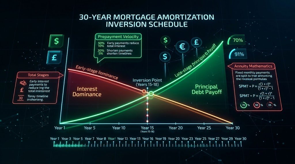
### 4.1 The Monthly Interest Calculation Law In each individual monthly payment cycle $k$: 1. The financial institution first computes the Accrued Interest ($I_k$) generated over the preceding 30 days against the remaining principal balance ($B_{k-1}$):

$$I_k = B_{k-1} \times r$$

2. The remaining portion of the monthly payment is then applied toward Principal Reduction ($P_k$):

$$P_k = PMT - I_k$$

3. The new remaining principal balance ($B_k$) for the subsequent month is updated:

$$B_k = B_{k-1} - P_k$$

### 4.2 The Reality of Early-Stage Interest Dominance Let us analyze the first payment cycle of our earlier $500,000 mortgage at 6.75% interest ($PMT = \$3,243.08$): - Initial Principal Balance ($B_0$): $500,000.00 - Monthly Interest Rate ($r$): $0.0675 / 12 = 0.005625$ - Month 1 Interest ($I_1$): $\$500,000 \times 0.005625 = \mathbf{\$2,812.50}$ - Month 1 Principal Paid ($P_1$): $\$3,243.08 - \$2,812.50 = \mathbf{\$430.58}$

Out of the borrower's $3,243.08 payment in Month 1, an astounding 86.7% ($2,812.50) is vaporized as pure bank profit and interest expense. A meager 13.3% ($430.58) actually reduces the debt.

### 4.3 The Amortization Inversion Point The Amortization Inversion Point is defined as the exact month $k^*$ where the principal reduction component surpasses the interest charge:

$$P_{k^*} > I_{k^*} \iff P_{k^*} > \frac{PMT}{2}$$

For a standard 30-year fixed loan at 6.75%, the Inversion Point does not occur until Month 203 (Year 17, Month 1). For the first 17 years of the mortgage, the borrower pays more interest than principal every single month.

If the borrower sells the property or refinances the loan at Year 7 (which is the statistical median tenure for US homeowners), they will have made 84 consecutive monthly payments totaling $\$272,418$. Yet, their remaining loan balance will still be approximately $\$453,800$. Over 7 full years of payments, they managed to retire only $\$46,200$ of principal.

Because monthly interest is calculated directly against the remaining outstanding balance ($B_{k-1}$), injecting additional capital directly into the principal pool produces an exponential multiplier effect. A single dollar paid toward principal today eliminates not just that dollar of debt, but also removes all future compound interest that dollar would have accumulated over the remaining decades of the loan term.

### 5.1 The Mathematical Impact of Prepayment When a borrower makes a supplemental principal prepayment $\Delta P$, the subsequent month's interest charge is permanently suppressed:

$$\Delta I_{k+1} = -\Delta P \times r$$

Because total monthly payment $PMT$ remains fixed, this permanent interest reduction cascades forward: every subsequent month, more of the base payment is automatically redirected into principal reduction, accelerating the debt retirement trajectory.

5.2 Comparative Analysis: Prepayment Scenarios on a $500,000 Mortgage (6.75% 30-Yr)

| Prepayment Strategy | Monthly Total Paid | Years to Payoff | Total Interest Paid | Lifetime Cash Savings | | :--- | :---: | :---: | :---: | :---: | | Standard Baseline (No extra payments) | $3,243.08 | 30.0 Years (360 mos) | $667,508 | $0 (Baseline) | | +$200 / Month Extra Principal | $3,443.08 | 25.2 Years (302 mos) | $538,210 | $129,298 saved | | +$500 / Month Extra Principal | $3,743.08 | 20.4 Years (245 mos) | $416,840 | $250,668 saved | | +$1,000 / Month Extra Principal | $4,243.08 | 15.6 Years (187 mos) | $302,490 | $365,018 saved | | Bi-Weekly Payment Strategy (26 half-payments/yr) | $1,621.54 / bi-wk | 24.1 Years (289 mos) | $512,180 | $155,328 saved |

### 5.3 The Bi-Weekly Mortgage Mechanism The Bi-Weekly Payment Strategy is an exceptionally popular and friction-free debt acceleration method. Instead of making 12 monthly payments of $PMT$, the borrower pays $\frac{PMT}{2}$ every two weeks.

Because there are 52 weeks in a calendar year, 52 bi-weekly intervals yield:

$$\text{Total Payments} = \frac{52}{2} = 26 \text{ half-payments} = 13 \text{ full monthly payments}$$

This strategy quietly executes one full extra monthly payment every year, applied directly to the principal balance without creating lifestyle disruption. On a $500,000 mortgage, this single optimization eliminates nearly 6 full years of debt and saves over $155,000 in cash interest.

While paying substantial compound interest is a severe financial drag, macroeconomic forces—specifically Monetary Inflation—can dramatically alter the real economic burden of fixed-rate long-term debt.

### 6.1 The Fisher Equation & The Real Cost of Borrowing Named after economist Irving Fisher, the Fisher Equation establishes the relationship between the nominal interest rate ($i$), the real interest rate ($r_{\text{real}}$), and expected inflation ($\pi$):

$$(1 + i) = (1 + r_{\text{real}})(1 + \pi)$$

Approximated in linear terms for moderate rates:

$$r_{\text{real}} \approx i - \pi$$

When an economy experiences elevated consumer price inflation (for example, $\pi = 5.5\%$) while a borrower holds a fixed-rate mortgage locked at $i = 6.75\%$, the Real Economic Interest Rate being paid on that debt is:

$$r_{\text{real}} = 6.75\% - 5.50\% = 1.25\%$$

The real cost of capital shrinks to near zero.

### 6.2 Debt Devaluation via Inflated Dollars Under a fixed-rate amortization contract, the monthly payment $PMT$ remains nominally locked for decades. If you borrow in 2026 with a $3,243 monthly payment, your payment in 2046 will still be precisely $3,243.

However, if general price levels and nominal wage earnings double over that 20-year span due to cumulative compounding inflation:

$$\text{Real Value of Month 240 Payment} = \frac{\$3,243}{(1 + \pi)^{20}} = \frac{\$3,243}{(1 + 0.035)^{20}} \approx \$1,630$$

In terms of real purchasing power, the borrower's payment burden is cut in half. The borrower is effectively repaying their 2026 debt using substantially depreciated, cheaper future currency units. This phenomenon explains why institutional real estate investors frequently prefer maintaining modest long-term fixed-rate leverage during inflationary eras rather than rushing to prepay low-cost capital.

For frontend software engineers building fintech platforms, loan origination portals, or in-browser financial calculators, the native JavaScript number type represents an insidious architectural hazard.

### 7.1 The IEEE 754 Binary Floating-Point Flaw JavaScript implements numbers using the IEEE 754 standard for double-precision binary floating-point (64-bit). In binary floating-point systems, decimal fractions (such as $0.1$ or $0.2$) cannot be represented with finite binary bits, resulting in repeating binary expansions:



If a banking application performs amortization calculations across 360 monthly iterations using naive JavaScript floating-point numbers, rounding errors compound at each step. By Month 360, the final loan balance will not equal $0.00; it will drift by several cents or even dollars, triggering critical audit compliance failures in enterprise financial systems.

### 7.2 The Integer Cents Pattern The simplest and most resilient architecture for handling monetary calculations without heavy third-party dependencies is the Integer Cents Pattern: never store currency amounts as fractional dollars. Instead, convert all monetary values to integer cents (or fractional hundredths of a cent) before performing additions, subtractions, and multiplications:



By encapsulating calculation logic within pure integer arithmetic and rounding specifically at the payment boundary, the schedule reconciles to exactly $\$0.00$ on the final payment date.

When managing multiple liabilities—such as student loans, credit card balances, auto loans, and residential mortgages—borrowers must deploy a disciplined debt reduction framework. In consumer financial engineering, two primary methodologies dominate: the Debt Avalanche Method and the Debt Snowball Method.

### 8.1 The Debt Avalanche Method (Pure Mathematical Optimization) The Debt Avalanche Method prioritizes debt repayment strictly in descending order of Interest Rate (APR), regardless of the principal balance amount.

1. Step 1: Make minimum scheduled payments on all liabilities to avoid credit score penalties and late fees. 2. Step 2: Direct 100% of available surplus cash flow toward the single loan carrying the highest nominal APR. 3. Step 3: Once the highest-APR debt is eliminated, roll its entire monthly cash allocation into the next highest-APR debt.

$$\text{Priority Order} = \arg\max_{\text{debt}} (\text{APR})$$

- Advantages: Minimizes total lifetime interest paid; mathematically guarantees the fastest possible path to net worth recovery. - Drawbacks: If the highest-rate loan has a massive balance, the borrower may go months or years without experiencing the psychological boost of closing an account.

### 8.2 The Debt Snowball Method (Behavioral Momentum Optimization) Popularized by personal finance authors, the Debt Snowball Method completely ignores interest rates and orders liabilities strictly in ascending order of Remaining Principal Balance.

1. Step 1: Pay minimum required installments across all credit facilities. 2. Step 2: Direct all surplus capital toward the smallest single balance. 3. Step 3: When that small balance is paid off, roll that cash flow into the next smallest debt.

$$\text{Priority Order} = \arg\min_{\text{debt}} (\text{Principal Balance})$$

- Advantages: Delivers rapid psychological victories and cognitive momentum; quickly reduces monthly required minimums. - Drawbacks: Sub-optimal from a pure mathematical perspective. Holding high-APR balances while paying off low-APR loans costs more total cash in cumulative interest.

### 8.3 The Hybrid Quantitative Strategy For high-income professionals and analytical engineers, the Hybrid Optimization Strategy offers the ideal balance: 1. Target and extinguish any predatory high-interest consumer debt ($> 12\%$ APR, such as credit cards or personal loans) using the Debt Avalanche Method. 2. For mid-tier collateralized debt ($5\%$ to $8\%$, such as mortgages or auto loans), establish a systematic Prepayment Schedule (e.g., adding 10% to 15% extra principal each month). 3. If low-cost fixed debt ($< 4\%$) was secured during historical low-rate eras, maintain standard amortization without early prepayment, investing surplus capital into diversified index funds yielding historical real returns of $7\%$ to $10\%$.

### Comprehensive Financial Action Plan: 1. Calculate your exact loan EMI using the mathematical annuity formula before signing lending contracts. 2. Examine the full 360-month amortization schedule to identify your specific Inversion Point. 3. Set up automated bi-weekly or monthly principal prepayments to dramatically slash lifetime interest expense. 4. Model high-inflation impacts to understand your real versus nominal debt liabilities. 5. Use client-side financial tools that ensure zero financial data is leaked across the internet.