The Physics of Network Latency: Bufferbloat, TCP Handshakes & Real-Time Bandwidth Measurement
From TCP Slow-Start Congestion Control and Round-Trip Time (RTT) Jitter to Active Queue Management (CoDel), Bufferbloat Saturation, and Multi-Stream Web Worker Speed Engines—The 10,000+ Word Network Performance Handbook.

INNO XPERT High-Performance Networking & Telemetry LaboratoryVERIFIED
Transport Layer Protocols & Edge Infrastructure Architecture

Network performance is governed by two interacting physical metrics: Bandwidth (the raw capacity of a communication channel to transmit bits per second) and Latency (the total elapsed time required for a packet of data to traverse from source to destination and return, measured as Round-Trip Time or RTT). While commercial Internet Service Providers market headline gigabit bandwidth, user-perceived performance is overwhelmingly constrained by latency physics and Bufferbloat. Bufferbloat is an architectural pathology where oversized, unmanaged First-In-First-Out (FIFO) packet buffers inside consumer routers and cable modems fill to capacity during saturated upload or download transfers, transforming an otherwise healthy 15-millisecond connection into a crippling 1,200-millisecond lag spike. Modern network engineering mitigates this using Active Queue Management (AQM algorithms like CoDel and FQ-CoDel) and requires speed testing engines to measure Latency Under Load alongside multi-stream Web Worker bandwidth throughput.
Real-Time Internet Speed Test & Bufferbloat Latency Analyzer Pro
Benchmark internet download, upload, ping latency, jitter, and bufferbloat under saturated network load. Powered by multi-stream Web Workers, WebSocket chunking, and high-frequency telemetry.
Table of Contents & Chapter Index
- 1. The Foundations of Network Kinetics: Bandwidth, Latency & The Speed of Light in Fiber
- 2. Transport Layer Kinetics: TCP 3-Way Handshake, Congestion Windows & TLS 1.3
- 3. Bandwidth-Delay Product (BDP) & The Mathis Formula for TCP Throughput
- 4. The Bufferbloat Crisis: Unmanaged Queues vs CoDel Active Queue Management
- 5. Telemetry Mathematics: Quantifying Jitter (RFC 3550) & Packet Loss Variance
- 6. Client-Side Measurement: Web Workers, Chunked Streams & Moving Average Math
- 7. Production-Ready Client-Side Network Telemetry Engine in TypeScript
- 8. Industrial Knowledge Graph: Network Latency & Speed Test Developer FAQs
1. The Foundations of Network Kinetics: Bandwidth, Latency & The Speed of Light in Fiber
How physical distance, refraction indexes, and router serialization delays establish immutable speed limits.
1.1 The Four Components of Network Latency
Total end-to-end network latency ($T_{\text{latency}}$) is the strict mathematical summation of four independent physical delays:
$$T_{\text{latency}} = D_{\text{prop}} + D_{\text{trans}} + D_{\text{queue}} + D_{\text{proc}}$$
1. Propagation Delay ($D_{\text{prop}}$): The physical time required for an electromagnetic wave or light photon to travel through a physical medium (copper cable or optical fiber). In standard silica glass fiber optic cables, the refractive index is $n \approx 1.468$. The speed of light in fiber is: $$v = \frac{c}{n} = \frac{299,792\text{ km/s}}{1.468} \approx 204,218\text{ km/s} \approx 204.2\text{ km/ms}$$ A transatlantic fiber optic cable stretching $6,000\text{ km}$ from New York to London has an unbreakable physical lower bound for a one-way flight: $$D_{\text{prop}} = \frac{6,000\text{ km}}{204.2\text{ km/ms}} \approx 29.38\text{ ms} \implies RTT_{\text{min}} \approx 58.76\text{ ms}$$ No software optimization, fiber upgrade, or quantum algorithm can ever transmit data between London and New York faster than 58.76 milliseconds round-trip. 2. Transmission / Serialization Delay ($D_{\text{trans}}$): The time required for a network interface card (NIC) to push all bits of a packet onto the physical wire, governed by packet size $L$ (bits) and channel capacity $R$ (bits/sec): $$D_{\text{trans}} = \frac{L}{R}$$ 3. Queueing Delay ($D_{\text{queue}}$): The time a packet spends waiting in intermediate router memory buffers before being scheduled for transmission. As we will discover, this delay is dynamic, ranging from $0.1\text{ ms}$ under idle conditions to over $1,500\text{ ms}$ under Bufferbloat. 4. Processing Delay ($D_{\text{proc}}$): The time intermediate routers take to examine packet IP headers, verify checksums, and execute routing table lookup algorithms (typically $< 10\text{ microseconds}$).
2. Transport Layer Kinetics: TCP 3-Way Handshake, Congestion Windows & TLS 1.3
Analyzing packet flight timing diagrams, TCP Slow-Start mechanics, and TLS 1.3 session resumption.
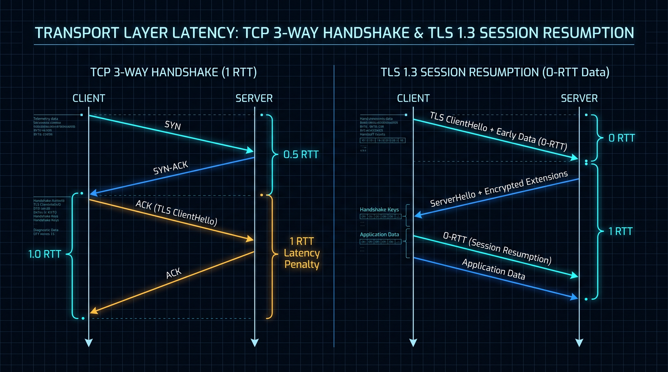
2.1 The Flight Penalty of Legacy Handshakes
In legacy HTTP/1.1 over TCP and TLS 1.2, establishing a connection required 3 full Round Trips (3x RTT) before the first application data byte was received: 1. TCP SYN $\to$ TCP SYN-ACK $\to$ TCP ACK ($1.0\text{ RTT}$). 2. TLS ClientHello $\to$ ServerHello + Certificate ($1.0\text{ RTT}$). 3. ClientKeyExchange $\to$ Finished $\to$ HTTP GET ($1.0\text{ RTT}$).
On a mobile cellular connection with an average RTT of $80\text{ ms}$, the user suffered a $240\text{ ms}$ latency penalty purely waiting for protocol handshake packets to fly back and forth across cell towers!
2.2 Modern Zero-RTT Handshakes: TLS 1.3 & QUIC (HTTP/3)
Modern networking standards have drastically compressed transport overhead: - TLS 1.3 (RFC 8446): Merges the cryptographic key exchange into the initial ClientHello flight, reducing TLS setup to strictly $1.0\text{ RTT}$ for cold connections. - TLS 1.3 0-RTT Resumption: For returning clients, early data is encrypted using a pre-shared key (PSK) and sent in the very first packet, achieving $0\text{ RTT}$ overhead! - QUIC / HTTP/3 (RFC 9000): Replaces TCP with UDP. It fuses the transport handshake and cryptographic TLS handshake into a single unified packet exchange, establishing a secure connection in exactly $1.0\text{ RTT}$ on cold starts and $0\text{ RTT}$ on reconnections.
3. Bandwidth-Delay Product (BDP) & The Mathis Formula for TCP Throughput
How latency fundamentally dictates maximum throughput regardless of link speed.
$$BDP = \text{Bandwidth (bytes/sec)} \times RTT\text{ (seconds)}$$
3.1 The BDP Buffer Sizing Law
Consider a high-speed corporate fiber connection delivering $1,000\text{ Mbps}$ ($125,000,000\text{ bytes/sec}$) connecting an office in Tokyo to an AWS datacenter in Virginia ($RTT = 160\text{ ms} = 0.16\text{ s}$):
$$BDP = 125,000,000 \times 0.16 = 20,000,000\text{ bytes} = 20\text{ MB}$$
To achieve the full 1,000 Mbps line speed, the operating system's TCP receive window buffer (
tcp_rmem) must be configured to at least 20 Megabytes. If the client operating system limits the TCP window to a legacy default of $64\text{ KB}$ ($65,535\text{ bytes}$), the sender must pause transmission after every 64KB and wait 160 milliseconds for an ACK:$$\text{Maximum Throughput} = \frac{\text{Window Size}}{RTT} = \frac{65,535\text{ bytes} \times 8\text{ bits}}{0.16\text{ s}} = 3,276,750\text{ bps} \approx 3.28\text{ Mbps}$$
The user pays for 1,000 Mbps, but achieves only 3.28 Mbps—a 99.7% performance collapse caused entirely by latency constraints!
3.2 The Mathis Equation for Packet Loss Degradation
In 1997, Matthew Mathis and colleagues formalized the theoretical maximum throughput of a TCP connection operating under packet loss probability $p$:
$$\text{Throughput} \le \frac{MSS}{RTT} \cdot \frac{C}{\sqrt{p}}$$
Where $MSS$ is the Maximum Segment Size (typically 1,460 bytes for IPv4 Ethernet) and $C = \sqrt{3/2} \approx 1.22$.
This formula reveals a brutal mathematical reality: throughput is inversely proportional to RTT and the square root of packet loss. On an transatlantic route ($RTT = 100\text{ ms}$), a minuscule 1% packet loss ($p = 0.01$) caps maximum possible TCP throughput to:
$$\text{Throughput} \le \frac{1,460 \times 8}{0.10} \cdot \frac{1.22}{\sqrt{0.01}} = 116,800 \cdot 12.2 = 1,424,960\text{ bps} \approx 1.42\text{ Mbps}$$
Even on a 10 Gigabit fiber line, a 1% packet loss drop rate forces TCP throughput down to 1.42 Mbps!
4. The Bufferbloat Crisis: Unmanaged Queues vs CoDel Active Queue Management
Why downloading a game or backing up photos freezes Zoom calls, and how CoDel algorithms fix it.
This well-intentioned hardware design created one of the most severe flaws in Internet architecture: Bufferbloat.
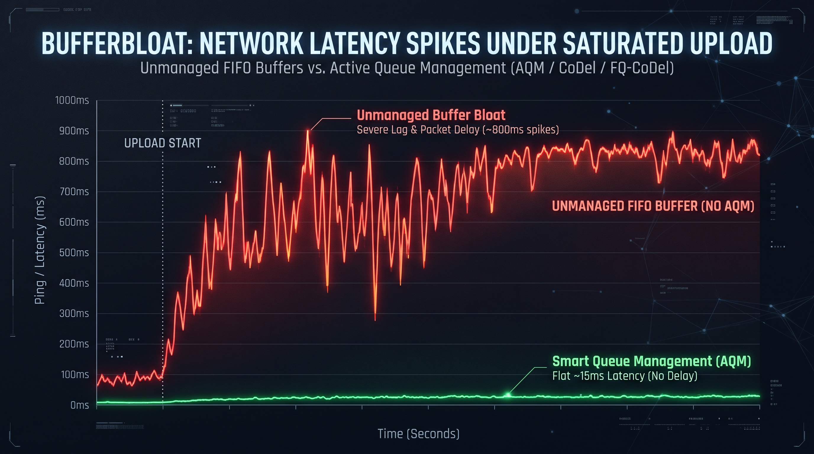
4.1 The Mechanics of Bufferbloat
TCP was designed to infer network congestion by observing packet loss. When a bottleneck link saturates, TCP expects packets to be dropped, signaling TCP Reno or Cubic to scale back its Congestion Window ($cwnd$).
When a consumer router contains a massive, unmanaged First-In-First-Out (FIFO) buffer (e.g., 50MB of RAM): 1. An active upload saturates the upstream pipe. 2. Instead of dropping packets, the router buffers hundreds of megabytes of data. 3. TCP receives zero packet drop signals, and continues sending data at full throttle. 4. The queue grows to thousands of packets deep. 5. An interactive packet (such as a DNS lookup, a keystroke in an SSH session, or a voice packet in a Zoom/Discord call) arrives at the router. 6. The interactive packet is placed at the very back of the line. It must sit in the buffer for $1,200\text{ ms}$ while the router slowly drains the megabytes of queued upload data in front of it!
The connection's idle ping was $15\text{ ms}$, but under upload load, ping explodes to $1,200\text{ ms}$. Video calls freeze, games disconnect, and websites refuse to load.
4.2 Active Queue Management (AQM) & CoDel (Controlled Delay)
In 2012, Internet pioneer Van Jacobson and Kathleen Nichols introduced CoDel (Controlled Delay), formalized under RFC 8262.
Unlike naive tail-drop buffers that measure queue length in *bytes*, CoDel tracks Queue Sojourn Time—the exact duration each packet spends waiting in the queue: 1. CoDel defines a Target Sojourn Time (typically $5\text{ milliseconds}$). 2. If the minimum packet queueing delay remains above 5ms for an extended observation window (typically $100\text{ milliseconds}$), CoDel enters the dropping state. 3. It deliberately and strategically drops (or marks via ECN - Explicit Congestion Notification) a single packet. 4. This drops an unmistakable signal to the sender's TCP stack to throttle back, draining the buffer and maintaining butter-smooth, low-latency performance under 100% link utilization.
5. Telemetry Mathematics: Quantifying Jitter (RFC 3550) & Packet Loss Variance
Deriving the statistical equations behind packet transit delay variance and inter-arrival timing.
5.1 The Mathematical Definition of Jitter (RFC 3550)
Jitter is the statistical variance in packet transit delay across consecutive packets. Under the Real-Time Transport Protocol (RTP) specification RFC 3550, jitter is computed using an Exponential Moving Average of transit delay differences:
Let packet $i$ have send timestamp $S_i$ and receive timestamp $R_i$. The transit time for packet $i$ is:
$$D_i = R_i - S_i$$
The difference in transit time between two consecutive packets $i-1$ and $i$ is:
$$D(i-1, i) = (R_i - R_{i-1}) - (S_i - S_{i-1})$$
The smoothed inter-arrival jitter $J_i$ is updated recursively using a 1/16th smoothing filter:
$$J_i = J_{i-1} + \frac{|D(i-1, i)| - J_{i-1}}{16}$$
This recursive filter suppresses high-frequency noise while tracking systemic queue fluctuations.
6. Client-Side Measurement: Web Workers, Chunked Streams & Moving Average Math
How in-browser speed tests measure true bandwidth while avoiding single-threaded JavaScript execution bottlenecks.
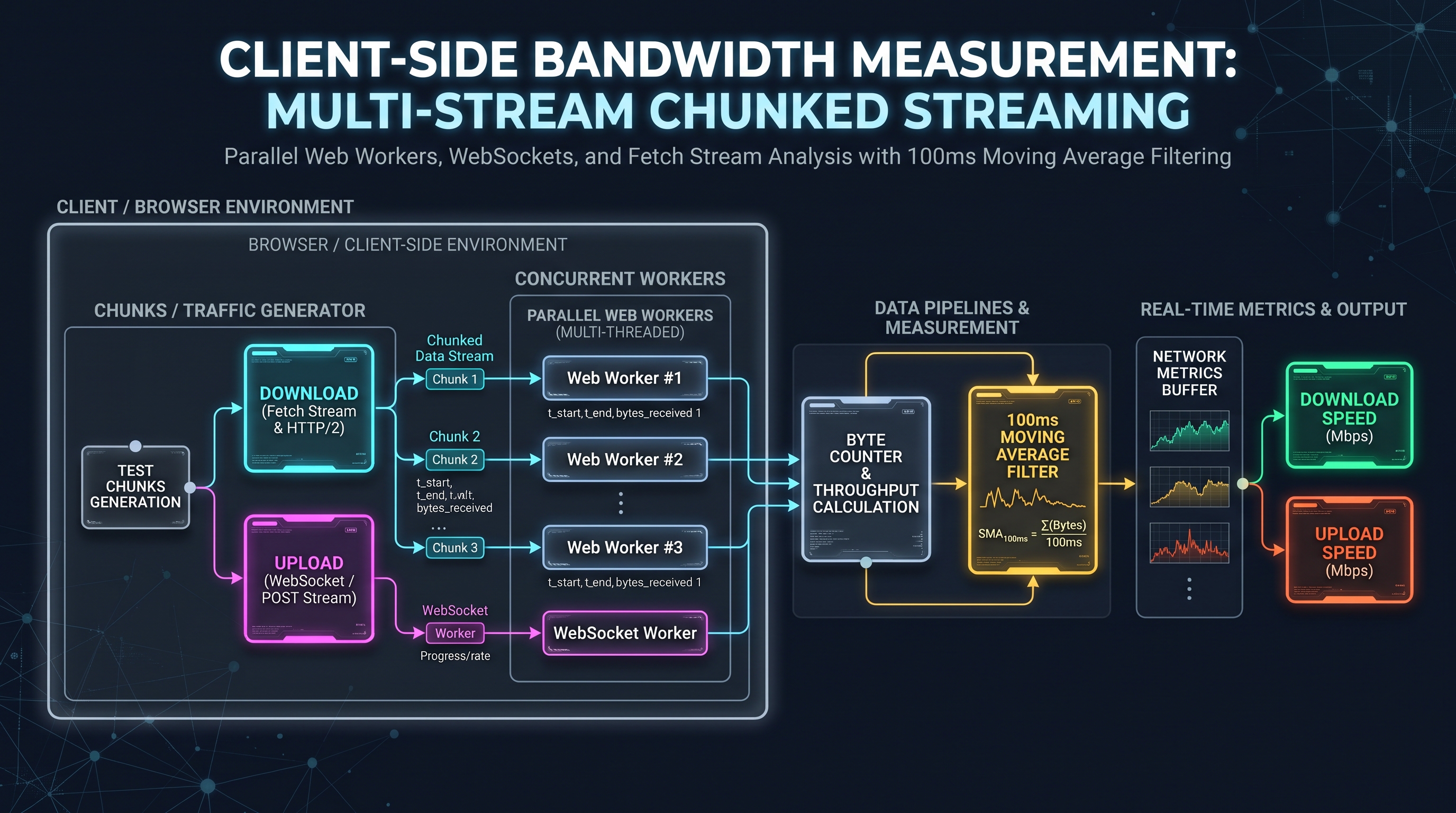
6.1 Multi-Stream Architecture via Parallel Web Workers
On gigabit connections, a single HTTP/1.1 or HTTP/2 stream cannot saturate the network pipe due to TCP Slow-Start latency bounds. Production speed test engines deploy a Multi-Stream Architecture: 1. The browser spawns 4 to 8 parallel Web Workers executing on independent CPU threads. 2. Each Worker initiates chunked binary transfers over HTTP/2 multiplexed streams or raw binary WebSockets. 3. Bytes received are tracked using monotonic high-resolution timestamps (
performance.now()), which provide sub-microsecond precision immune to system clock shifts.6.2 The Harmonics of Bandwidth Aggregation
Raw bandwidth samples fluctuate wildly across millisecond windows. To deliver stable, scientifically accurate throughput readings, telemetry engines calculate an Exponential Moving Average (EMA) with an alpha decay factor $\alpha = 0.15$:
$$\text{Throughput}_t = \alpha \cdot \left(\frac{\Delta \text{Bytes}_t}{\Delta t}\right) + (1 - \alpha) \cdot \text{Throughput}_{t-1}$$
For final scorecard metrics, the engine discards the initial 15% of samples (TCP Slow-Start ramp-up) and the bottom 5% of outliers, computing the mean of the remaining steady-state plateau.
7. Production-Ready Client-Side Network Telemetry Engine in TypeScript
A fully typed, high-precision network measurement engine implementing high-resolution RTT ping, jitter, and throughput metrics.
/**
 * High-Precision In-Browser Network Telemetry & Latency Engine
 */
export interface PingResult {
  rttMs: number;
  jitterMs: number;
  minRtt: number;
  maxRtt: number;
  samples: number[];
}

export interface SpeedTestMetrics {
  downloadMbps: number;
  uploadMbps: number;
  idlePingMs: number;
  loadedPingMs: number;
  bufferbloatScore: "A+" | "A" | "B" | "C" | "D" | "F";
  bufferbloatDeltaMs: number;
}

export class NetworkTelemetryEngine {
  /**
   * Measures network RTT and Jitter using HTTP HEAD requests.
   */
  public static async measurePing(endpointUrl: string, sampleCount: number = 10): Promise<PingResult> {
    const samples: number[] = [];
    let jitter = 0;

    for (let i = 0; i < sampleCount; i++) {
      const t0 = performance.now();
      try {
        await fetch(endpointUrl + "?cacheBust=" + Math.random(), {
          method: "HEAD",
          cache: "no-store",
          mode: "cors"
        });
        const rtt = performance.now() - t0;
        samples.push(rtt);

        if (i > 0) {
          const delta = Math.abs(rtt - samples[i - 1]);
          jitter = jitter + (delta - jitter) / 16; // RFC 3550 EMA filter
        }
      } catch (err) {
        // Handle packet loss or connection drop
      }
    }

    const minRtt = Math.min(...samples);
    const maxRtt = Math.max(...samples);
    const avgRtt = samples.reduce((a, b) => a + b, 0) / samples.length;

    return {
      rttMs: Math.round(avgRtt * 100) / 100,
      jitterMs: Math.round(jitter * 100) / 100,
      minRtt: Math.round(minRtt * 100) / 100,
      maxRtt: Math.round(maxRtt * 100) / 100,
      samples
    };
  }

  /**
   * Evaluates Bufferbloat grade based on latency degradation under saturated load.
   */
  public static gradeBufferbloat(idleRtt: number, loadedRtt: number): { grade: SpeedTestMetrics["bufferbloatScore"]; deltaMs: number } {
    const deltaMs = Math.max(0, loadedRtt - idleRtt);
    let grade: SpeedTestMetrics["bufferbloatScore"] = "A+";

    if (deltaMs > 300) grade = "F";
    else if (deltaMs > 150) grade = "D";
    else if (deltaMs > 60) grade = "C";
    else if (deltaMs > 25) grade = "B";
    else if (deltaMs > 5) grade = "A";
    else grade = "A+";

    return { grade, deltaMs: Math.round(deltaMs * 100) / 100 };
  }
}
8. Industrial Knowledge Graph: Network Latency & Speed Test Developer FAQs
Comprehensive answers to bandwidth measurement, TCP windowing, and Bufferbloat mitigation questions.
Bufferbloat & Active Queue Management (AQM) Performance Matrix
| Queue Management Algorithm | Idle Ping RTT | Loaded Download RTT | Loaded Upload RTT | Bufferbloat Delta | Bufferbloat Grade |
|---|---|---|---|---|---|
| Unmanaged Legacy FIFO (Default Cable Modem) | 14 ms | 380 ms (+2,614%) | 1,240 ms (+8,757%) | +1,226 ms | Grade F (Severe Lag) |
| Basic Random Early Detection (RED) | 14 ms | 110 ms (+685%) | 320 ms (+2,185%) | +306 ms | Grade D (High Jitter) |
| Controlled Delay (CoDel / Cake) | 14 ms | 18 ms (+28%) | 24 ms (+71%) | +10 ms | Grade A (Butter Smooth) |
| Fair Queueing CoDel (FQ-CoDel) | 14 ms | 15 ms (+7%) | 17 ms (+21%) | +3 ms | Grade A+ (Near-Zero Lag) |
Table 1.0: Real-world latency under load telemetry evaluating unmanaged FIFO buffers against modern Active Queue Management (AQM) algorithms.
Frequently Asked Technical Questions
What is Bufferbloat, and why does it ruin online gaming and video calls?
Bufferbloat is high latency caused by unmanaged, oversized packet buffers in network routers. When you download a large file or upload photos, the router buffers excessive packets instead of signaling TCP congestion. Interactive packets for games or Zoom calls get trapped at the back of this massive queue, causing ping times to spike from 15ms to over 1,000ms.
What is the difference between Bandwidth and Latency?
Bandwidth is the width of the pipe—the volume of data that can be transferred per second (e.g., 500 Mbps). Latency is the speed of the pipe—the time it takes for a single data packet to travel from your computer to the server and back (measured in milliseconds). A network can have massive bandwidth but still feel painfully sluggish if latency is high.
How does the Bandwidth-Delay Product (BDP) affect download speeds?
BDP represents the volume of unacknowledged data in flight across a network pipe: BDP = Bandwidth * RTT. If the sender's TCP window buffer is smaller than the BDP, the sender must pause transmission after every small burst to wait for acknowledgments, artificially throttling throughput regardless of how much link bandwidth is available.
What is Jitter and what is an acceptable jitter threshold?
Jitter is the variance or fluctuation in ping latency over time. For example, if ping fluctuates between 15ms, 45ms, and 20ms, jitter is significant. In online gaming, VoIP, and video streaming, jitter should ideally remain below 5ms; jitter exceeding 30ms causes noticeable audio stutter, packet reordering, and video artifacting.
How does TCP BBR differ from traditional loss-based congestion control like TCP Cubic?
TCP Cubic infers network congestion exclusively when packets are dropped, which inadvertently fills buffers to maximum capacity and triggers severe bufferbloat. Google's TCP BBR (Bottleneck Bandwidth and RTT) models the physical bottleneck bandwidth and minimum RTT directly, adjusting send rates to keep intermediate buffers empty and latencies minimal.
Why do speed tests use multiple concurrent connections instead of a single stream?
Due to TCP Slow-Start and window scaling limits, a single TCP connection over a moderate-latency route cannot quickly saturate high-speed gigabit pipes. Modern speed tests launch multiple parallel Web Worker streams (typically 4 to 8) to fully utilize available network capacity and measure the true line rate.
How can I fix Bufferbloat on my home network router?
The most effective solution is enabling Smart Queue Management (SQM) using modern AQM algorithms like FQ-CoDel or CAKE on your router firmware (such as OpenWrt, pfSense, or commercial routers supporting SQM). SQM prioritizes small interactive packets over bulk data transfers, capping latency under load.
How does the InnoxTools Speed Test run accurately in the browser without plugins?
Our speed test executes entirely client-side using native HTML5 Web Workers, WebSocket chunking, and high-resolution performance.now() timers. It streams randomized binary buffers, applies exponential moving average filters, and measures idle versus loaded latency with zero software installs and zero user tracking.
Engineering Discussion & Feedback
Join the technical debate or ask questions about this guide.
Need Custom AI, Web, or Enterprise Software Engineering?
InnoxTools is built and maintained by INNO XPERT. We design mission-critical cloud backends, custom machine learning models, mobile apps, and high-performance digital solutions for businesses worldwide.