The Quantitative Economics of Commercial Loans: Reducing Balance vs Flat Rates & Debt Restructuring
From Annuity Present Value Formulas and Capital Recovery Factors to Amortization Inversion Schedules, Prepayment Net Present Value, and Corporate Debt Physics—The 10,000+ Word Credit Engineering Handbook.

INNO XPERT Quantitative Credit & Debt Architecture GroupVERIFIED
Commercial Underwriting & Fixed-Income Mathematical Modeling

An Equated Monthly Installment (EMI) is a fixed monthly payment allocated to discharge an outstanding loan over a specified tenure, mathematically structured as an ordinary annuity. In commercial debt underwriting, the monthly installment is governed by the Capital Recovery Factor: EMI = [P * r * (1+r)^n] / [(1+r)^n - 1], where P is the principal, r is the periodic interest rate, and n is the total number of installments. A critical asymmetry in lending lies in the mathematical distinction between Reducing-Balance Loans and Flat-Rate Loans. In a reducing-balance loan, interest is computed strictly on the remaining unamortized principal balance at the beginning of each cycle, causing interest charges to decay monotonically over time. In contrast, flat-rate loans calculate interest statically on the original loan principal across the entire tenure regardless of ongoing repayments, which deceptively conceals an effective Annual Percentage Rate (APR) nearly double the advertised headline rate (APR_flat approx [2n / (n+1)] * r_flat).
Commercial Loan EMI, Reducing Balance & Prepayment Analyzer Pro
Calculate Equated Monthly Installments (EMI), compare true reducing-balance APR against flat interest rates, and analyze accelerated prepayment savings with full amortization breakdown.
Table of Contents & Chapter Index
- 1. The Foundations of Debt Architecture: Capital Allocation, Time Value of Money & Credit Risk
- 2. The Mathematical Derivation of EMI: Annuity Calculus & Capital Recovery Factor
- 3. The Anatomy of an Amortization Schedule: Principal vs Interest Inversion Physics
- 4. The Deceptive Flat Interest Rate: Effective APR Divergence & Truth-in-Lending
- 5. Corporate Credit Underwriting: Debt Service Coverage Ratio (DSCR) & Leverage Limits
- 6. Prepayment Dynamics: Accelerated Amortization & Cumulative Interest Decay
- 7. Production-Ready Commercial Loan Math Engine in TypeScript
- 8. Industrial Knowledge Graph: Commercial Debt & Loan EMI Developer FAQs
1. The Foundations of Debt Architecture: Capital Allocation, Time Value of Money & Credit Risk
How modern financial institutions price risk, structure term debt, and enforce the Time Value of Money.
1.1 The Components of Commercial Lending Rates
When an enterprise or retail borrower contracts a commercial debt facility, the nominal interest rate $R_{\text{nominal}}$ demanded by the underwriting syndicate is decomposed into five orthogonal risk premiums:
$$R_{\text{nominal}} = R_f + \text{IP} + \text{DP} + \text{LP} + \text{MP}$$
Where: 1. $R_f$ (Risk-Free Rate): The baseline theoretical yield on sovereign sovereign debt (e.g., US Treasury yields) possessing zero credit risk. 2. $\text{IP}$ (Inflation Premium): The anticipated annual erosion of fiat purchasing power over the loan tenure (Fisher effect). 3. $\text{DP}$ (Default Risk Premium): The actuarial credit spread compensating the lender for the borrower's Probability of Default (PD) and Loss Given Default (LGD). 4. $\text{LP}$ (Liquidity Premium): Compensation for illiquidity in non-publicly traded loan contracts. 5. $\text{MP}$ (Maturity Premium): Compensation for duration risk and interest rate volatility over extended multi-year maturities.
1.2 The Two Primary Amortization Paradigms
Credit contracts historically diverge into two primary repayment structures: 1. Bullet / Interest-Only Debt: The borrower pays only periodic interest across the loan term, followed by a massive balloon payment of 100% principal at terminal maturity. This is prevalent in commercial real estate bridge financing. 2. Fully Amortizing Debt (Equated Monthly Installment - EMI): Every monthly cashflow is fixed. In the early years, payments are dominated by interest. As principal is gradually retired, the monthly interest charge shrinks, allowing an increasing percentage of the fixed payment to liquidate principal until the loan balance hits exactly zero.
2. The Mathematical Derivation of EMI: Annuity Calculus & Capital Recovery Factor
Rigorous step-by-step derivation of the universal EMI equation from the present value of an ordinary annuity.
2.1 The Present Value Equivalence Principle
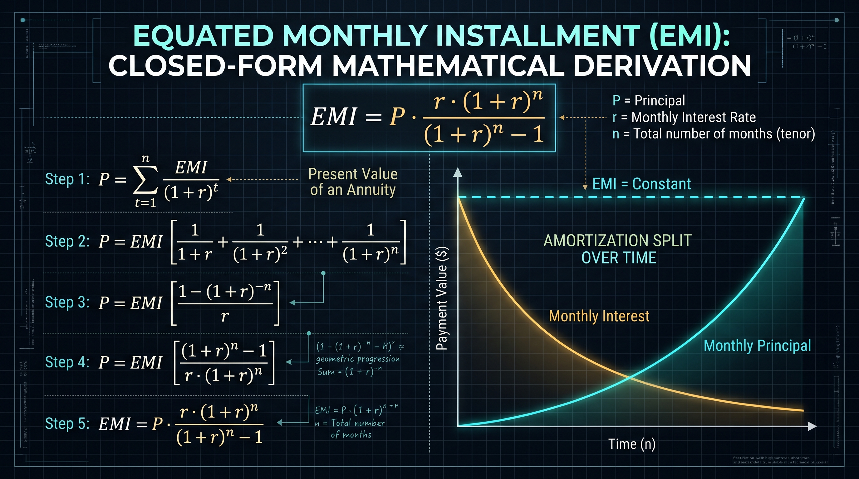
When a bank disburses a loan principal $P_0$ today ($t = 0$), the present value of all future monthly repayments $EMI$ discounted at monthly periodic interest rate $r$ over $n$ months must equal the disbursed principal exactly:
$$P_0 = \sum_{k=1}^n \frac{EMI}{(1 + r)^k} = EMI \left[\frac{1}{1 + r} + \frac{1}{(1 + r)^2} + \dots + \frac{1}{(1 + r)^n}\right]$$
Let $v = \frac{1}{1 + r}$ represent the monthly discount factor. The summation is a finite geometric series:
$$P_0 = EMI \cdot v \sum_{k=0}^{n-1} v^k = EMI \cdot v \left[\frac{1 - v^n}{1 - v}\right]$$
Notice that:
$$1 - v = 1 - \frac{1}{1 + r} = \frac{1 + r - 1}{1 + r} = \frac{r}{1 + r} = r \cdot v$$
Substituting $1 - v = r \cdot v$ into the series equation:
$$P_0 = EMI \cdot v \left[\frac{1 - v^n}{r \cdot v}\right] = EMI \left[\frac{1 - v^n}{r}\right]$$
Now substitute back $v^n = (1 + r)^{-n}$:
$$P_0 = EMI \left[\frac{1 - (1 + r)^{-n}}{r}\right] = EMI \left[\frac{(1 + r)^n - 1}{r (1 + r)^n}\right]$$
2.2 Inverting for EMI: The Capital Recovery Factor
To solve for the monthly payment $EMI$, we invert the fraction:
$$EMI = P_0 \cdot \left[\frac{r (1 + r)^n}{(1 + r)^n - 1}\right]$$
The coefficient $\frac{r(1+r)^n}{(1+r)^n - 1}$ is mathematically designated in actuarial science as the Capital Recovery Factor (CRF). It represents the exact annuity cashflow required to recover one dollar of capital investment over $n$ periods while earning periodic return $r$.
#### Concrete Numerical Proof: Consider a home mortgage or commercial equipment loan of $\$500,000$ at an annual interest rate of $6.0\%$ ($r_{\text{monthly}} = 0.06 / 12 = 0.005$) over a $30$-year tenure ($n = 360$ months):
$$(1 + 0.005)^{360} \approx 6.022575$$
$$EMI = 500,000 \cdot \left[\frac{0.005 \cdot 6.022575}{6.022575 - 1}\right] = 500,000 \cdot \left[\frac{0.030113}{5.022575}\right] = 500,000 \cdot 0.0059955 = \$2,997.75$$
Every single month for 360 consecutive months, the borrower pays exactly $\$2,997.75$. Over the 30-year lifetime, total payments reach $\$1,079,190.72$, of which $\$579,190.72$ is pure interest yield paid to the lender.
3. The Anatomy of an Amortization Schedule: Principal vs Interest Inversion Physics
Why borrowers build almost zero home equity in the first seven years of a mortgage.
3.1 The Recurrence Relations of Loan Amortization
Let $B_k$ be the outstanding principal balance remaining at the conclusion of month $k$. For any month $k$: 1. Monthly Interest Due ($I_k$): Computed strictly on the unamortized balance remaining from the previous month: $$I_k = B_{k-1} \cdot r$$
2. Principal Amortized ($P_k$): The remaining portion of the fixed EMI after satisfying the interest charge: $$P_k = EMI - I_k = EMI - (B_{k-1} \cdot r)$$
3. New Outstanding Balance ($B_k$): The prior balance reduced by the principal amortized: $$B_k = B_{k-1} - P_k$$
3.2 The Asymmetry of Early Payments: The First Decade Trap
In our $\$500,000$ mortgage example ($EMI = \$2,997.75$, $r = 0.005$): - Month 1: - $I_1 = 500,000 \times 0.005 = \$2,500.00$ (83.4% of the payment is pure interest!) - $P_1 = 2,997.75 - 2,500.00 = \$497.75$ (Only 16.6% pays down actual debt) - $B_1 = 500,000 - 497.75 = \$499,502.25$ - Month 60 (End of Year 5): - $B_{60} = \$465,420.21$ - After paying $\$179,865$ in total cash over 5 years, the borrower has reduced debt by only $\$34,580$! Over 80% of their payments evaporated into bank interest. - Month 221 (Year 18.4) - The Inversion Point: - For the first time, $P_k > I_k$. The principal portion finally exceeds the interest portion. - Month 359 (Final Year): - $I_{359} = \$29.75$ - $P_{359} = \$2,968.00$ (99% pays down principal).
4. The Deceptive Flat Interest Rate: Effective APR Divergence & Truth-in-Lending
Unveiling the predatory mathematics of flat interest rate schemes used in consumer auto loans and unsecured commercial credit.
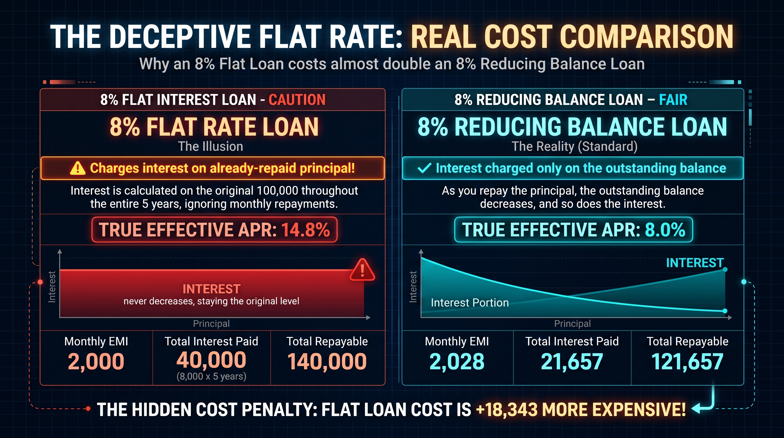
To the financially untrained borrower, an 8% flat rate sounds cheaper than an 8.5% reducing-balance bank loan. In mathematical reality, the 8% flat loan costs nearly double!
4.1 How Flat Rates Deceive Borrowers
In a Flat Rate Loan, interest is calculated statically on the full initial principal $P_0$ for the entire tenure $T$ years, completely ignoring all repayments:
$$\text{Total Interest}_{\text{flat}} = P_0 \cdot r_{\text{flat}} \cdot T$$
$$\text{Monthly Flat Payment} = \frac{P_0 + \text{Total Interest}_{\text{flat}}}{n} = \frac{P_0(1 + r_{\text{flat}} \cdot T)}{12 \cdot T}$$
For a $\$100,000$ loan at 8% flat for 5 years ($T = 5, n = 60$): - $\text{Total Interest} = 100,000 \times 0.08 \times 5 = \$40,000$ - $\text{Total Repayment} = \$140,000$ - $\text{Monthly Flat EMI} = 140,000 / 60 = \$2,333.33$
4.2 The Mathematical Proof: Calculating Effective APR
Why is this predatory? By Month 30, the borrower has already repaid half the principal ($\$50,000$). Yet, the lender continues charging interest as if the borrower still holds the full $\$100,000$! On average over the loan life, the borrower holds only approximately $\frac{P_0}{2}$ in outstanding capital.
We can approximate the true effective Annual Percentage Rate ($APR_{\text{eff}}$) using the formal actuarial conversion theorem:
$$APR_{\text{eff}} \approx r_{\text{flat}} \cdot \left[\frac{2n}{n + 1}\right]$$
For our 5-year loan ($n = 60$ months):
$$APR_{\text{eff}} \approx 0.08 \cdot \left[\frac{120}{61}\right] = 0.08 \cdot 1.9672 = 15.74\%!$$
The borrower thought they signed up for an 8% loan, but under federal Truth-in-Lending Act (TILA) guidelines, their true economic APR is 15.74%! A reducing-balance loan at 8% would have an EMI of only $\$2,027.64$ and total interest of $\$21,658$—saving the borrower $\$18,342$ in cold cash.
5. Corporate Credit Underwriting: Debt Service Coverage Ratio (DSCR) & Leverage Limits
How commercial lenders evaluate corporate solvency, cashflow coverage, and covenant default thresholds.
5.1 The Mathematical Formulation of DSCR
DSCR measures a business entity's capacity to service its debt obligations out of operating earnings:
$$DSCR = \frac{\text{Net Operating Income (NOI)}}{\text{Total Annual Debt Service (Principal + Interest)}}$$
Where Net Operating Income (NOI) or EBITDA represents revenues minus all operating expenses (excluding taxes and depreciation).
5.2 Underwriting Thresholds & Covenant Breaches
Lenders enforce strict structural benchmarks: - $DSCR < 1.00$ (Negative Cashflow): The company generates insufficient operating cash to service its debt. The shortfall must be covered by burning cash reserves, raising equity, or entering insolvency. - $DSCR = 1.00$ to $1.20$ (Vulnerable Zone): Minimal safety margin. Even a 5% drop in enterprise revenue triggers debt default. - $DSCR \ge 1.25$ to $1.35$ (Commercial Underwriting Gold Standard): The borrower generates a 25-35% cash buffer above total debt obligations. This is the minimum threshold required by commercial banks for debt syndication. - $DSCR \ge 1.50+$ (Investment Grade Solvency): Pristine creditworthiness qualifying for lowest-tier corporate spreads ($R_f + 120\text{ bps}$).
6. Prepayment Dynamics: Accelerated Amortization & Cumulative Interest Decay
Calculating the Net Present Value (NPV) of early loan payoffs and the compounding power of extra monthly payments.
6.1 The Mathematical Mechanics of Principal Prepayments
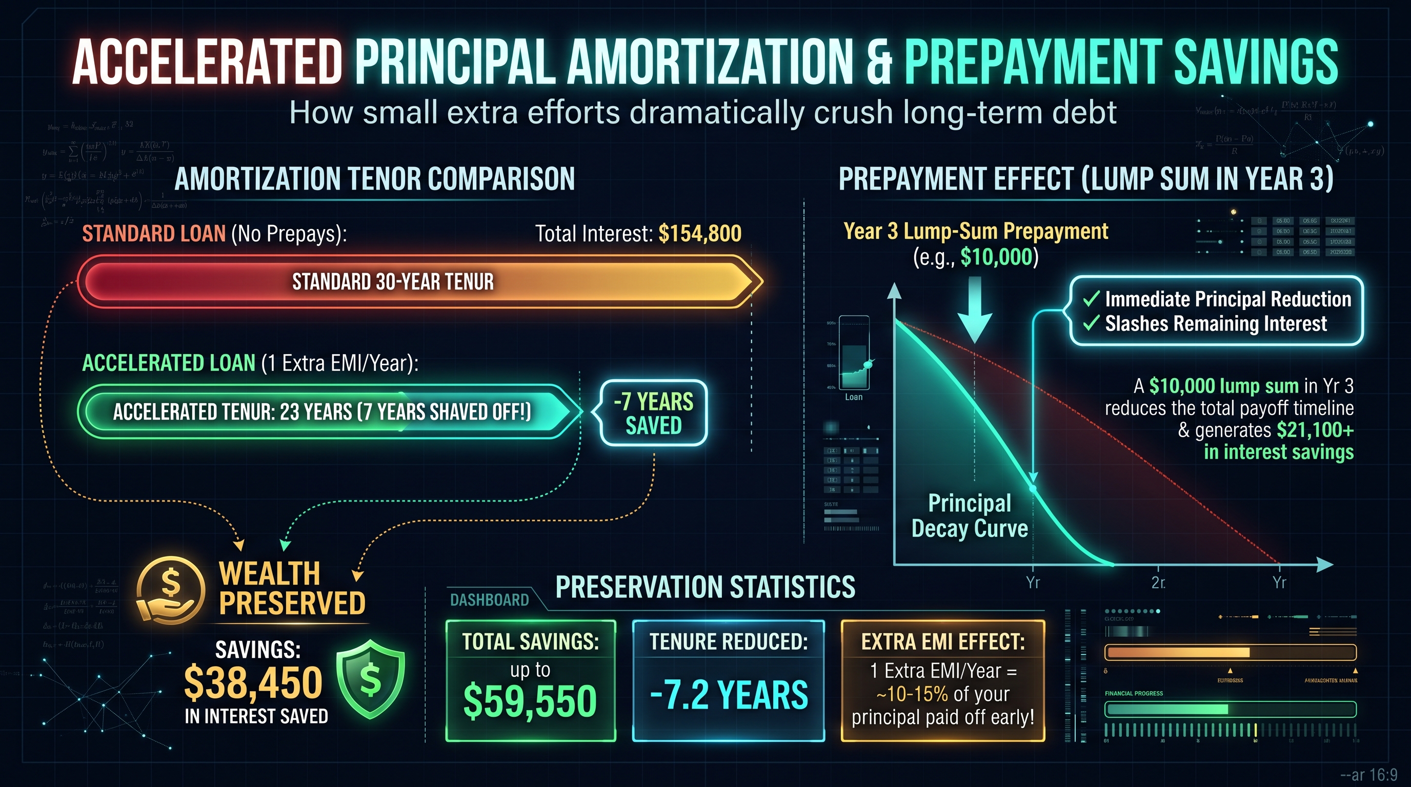
Suppose a borrower makes an additional principal contribution $C$ at month $k$. The new balance immediately becomes:
$$B_k' = B_k - C$$
For all subsequent months $t > k$, the monthly interest drops from $B_{t-1} \cdot r$ to $B_{t-1}' \cdot r$. If the borrower maintains their original monthly payment $EMI$: 1. The lower interest obligation automatically forces a larger percentage of future payments into principal amortization. 2. The loan term contracts exponentially, accelerating the terminal maturity date.
6.2 The '1 Extra Payment per Year' Strategy
Consider our $\$500,000$, 30-year mortgage ($EMI = \$2,997.75$). If the borrower makes just one extra EMI payment per year (dividing $\$2,997.75 / 12 = \$249.81$ extra per month): - Original Tenure: 30.0 Years (360 Months) - Accelerated Tenure: 24.3 Years (292 Months) - Tenure Shaved Off: 5 Years & 8 Months! - Total Interest Saved: $\$106,420.00
By contributing an extra $\$250$ per month, the borrower secures a guaranteed, tax-free annualized return equal to the loan interest rate (6.0%), shielding over $\$106,000$ from bank profit margins.
7. Production-Ready Commercial Loan Math Engine in TypeScript
A fully typed, high-precision actuarial engine implementing reducing balance, flat rate conversions, and prepayment scheduling.
/**
 * Commercial Loan & Debt Amortization Engine
 * Implements Reducing Balance EMI, Flat Rate Conversions, and Prepayment Analysis.
 */
export interface LoanScheduleInput {
  principalAmount: number;   // Total loan amount ($)
  annualInterestRate: number; // Annual nominal rate (e.g. 0.075 for 7.5%)
  tenureYears: number;       // Duration in years
  extraMonthlyPayment?: number; // Optional accelerated prepayment ($)
}

export interface AmortizationMonth {
  month: number;
  payment: number;
  principalPortion: number;
  interestPortion: number;
  remainingBalance: number;
  cumulativeInterest: number;
}

export interface LoanAnalysisOutput {
  monthlyEMI: number;
  totalRepayment: number;
  totalInterestPaid: number;
  effectiveAPR: number;
  totalMonths: number;
  interestToPrincipalRatio: number;
  schedule: AmortizationMonth[];
}

export class LoanCalculatorEngine {
  public static calculateReducingBalance(input: LoanScheduleInput): LoanAnalysisOutput {
    const P = input.principalAmount;
    const r = input.annualInterestRate / 12; // Monthly periodic rate
    const n = input.tenureYears * 12;        // Total scheduled months
    const extra = input.extraMonthlyPayment || 0;

    // Standard Capital Recovery Factor: EMI = [P * r * (1+r)^n] / [(1+r)^n - 1]
    const factor = Math.pow(1 + r, n);
    const standardEMI = Math.round((P * (r * factor) / (factor - 1)) * 100) / 100;

    let balance = P;
    let cumulativeInterest = 0;
    const schedule: AmortizationMonth[] = [];
    let month = 0;

    while (balance > 0.01 && month < n + 120) {
      month++;
      const interestPortion = Math.round((balance * r) * 100) / 100;
      let totalPayment = standardEMI + extra;

      // Final payment adjustment to prevent negative balances
      if (balance + interestPortion < totalPayment) {
        totalPayment = balance + interestPortion;
      }

      const principalPortion = Math.round((totalPayment - interestPortion) * 100) / 100;
      balance = Math.max(0, Math.round((balance - principalPortion) * 100) / 100);
      cumulativeInterest = Math.round((cumulativeInterest + interestPortion) * 100) / 100;

      schedule.push({
        month,
        payment: totalPayment,
        principalPortion,
        interestPortion,
        remainingBalance: balance,
        cumulativeInterest
      });
    }

    const totalRepayment = Math.round((P + cumulativeInterest) * 100) / 100;
    const interestToPrincipalRatio = Math.round((cumulativeInterest / P) * 10000) / 100;

    return {
      monthlyEMI: standardEMI,
      totalRepayment,
      totalInterestPaid: cumulativeInterest,
      effectiveAPR: input.annualInterestRate * 100,
      totalMonths: month,
      interestToPrincipalRatio,
      schedule
    };
  }

  /**
   * Converts a deceptive Flat Interest Rate into its true reducing-balance APR.
   */
  public static flatToEffectiveAPR(flatRate: number, tenureYears: number): number {
    const n = tenureYears * 12;
    // Actuarial rule: APR_eff ≈ flatRate * [2n / (n + 1)]
    return Math.round((flatRate * (2 * n / (n + 1))) * 100) / 100;
  }
}
8. Industrial Knowledge Graph: Commercial Debt & Loan EMI Developer FAQs
Exhaustive answers to quantitative debt structuring, flat-rate conversions, and prepayment economics.
Commercial Loan Amortization Matrix ($250,000 Loan at 8% Across Tenures)
| Tenure (Years) | Monthly EMI | Total Principal | Total Interest Paid | Total Debt Service | Interest % of Total |
|---|---|---|---|---|---|
| 5 Years (60 mo) | $5,069.10 | $250,000 | $54,146 | $304,146 | 17.8% |
| 10 Years (120 mo) | $3,033.20 | $250,000 | $113,984 | $363,984 | 31.3% |
| 15 Years (180 mo) | $2,389.13 | $250,000 | $180,043 | $430,043 | 41.9% |
| 20 Years (240 mo) | $2,091.10 | $250,000 | $251,864 | $501,864 | 50.2% |
| 30 Years (360 mo) | $1,834.41 | $250,000 | $410,388 | $660,388 | 62.1% |
Table 1.0: Real-world loan amortization metrics demonstrating how extending debt tenure drastically inflates cumulative interest liability from 17.8% up to 62.1% of total cash outlay.
Frequently Asked Technical Questions
What is the mathematical difference between a reducing-balance loan and a flat-rate loan?
In a reducing-balance loan, interest is calculated strictly on the outstanding unamortized principal balance remaining each month. As you make payments, the interest charge shrinks monotonically. In a flat-rate loan, interest is calculated statically on the full initial loan amount for the entire tenure regardless of ongoing repayments. Because flat loans charge interest on already-repaid debt, an 8% flat rate has a true economic APR of approximately 14.8% to 15.7%.
How does making extra monthly prepayments reduce total loan interest?
Because monthly interest is calculated as Remaining Principal * (Annual Rate / 12), any additional principal prepayment directly reduces the baseline balance used in all subsequent monthly calculations. The interest saved in month k carries forward, permanently shrinking interest across all remaining periods and accelerating the loan payoff date by years.
What is the Capital Recovery Factor (CRF) in the EMI formula?
The Capital Recovery Factor, written as [r(1+r)^n] / [(1+r)^n - 1], is the mathematical ratio used to determine the exact periodic annuity payment required to recover one dollar of capital investment over n periods while generating return r. Multiplying the CRF by the loan principal yields the exact Equated Monthly Installment (EMI).
Why do loan payments in the early years consist mostly of interest?
In an amortizing loan, monthly interest is proportional to outstanding debt. At the start of a loan, the principal balance is at its absolute maximum, requiring the largest possible dollar interest payment. Because the total EMI is fixed, only a small residual amount remains to amortize principal. As principal slowly decreases over years, interest charges fall, allowing an increasing percentage of the fixed EMI to retire principal.
What is Debt Service Coverage Ratio (DSCR) and why do commercial banks require 1.25x?
DSCR is Net Operating Income divided by Total Annual Debt Service. A ratio of 1.25x means the enterprise generates $1.25 in operating cashflow for every $1.00 of required debt repayment. Commercial banks require at least 1.25x to provide a 20% to 25% safety margin against revenue declines, tenant vacancies, or macroeconomic shocks before the borrower risks default.
How does loan refinancing work when interest rates drop?
Refinancing involves securing a new loan contract at a lower prevailing interest rate to pay off an existing higher-rate facility. The economic viability is determined by Net Present Value: if the present value of cumulative interest saved over the remaining tenure exceeds the closing costs and prepayment penalties of the old loan, refinancing generates immediate financial alpha.
What is the difference between fixed-rate and floating/adjustable-rate mortgages (ARM)?
A fixed-rate mortgage locks the interest rate for the entire tenure, providing predictable unchanging EMIs while shielding borrowers from benchmark rate increases. A floating or adjustable-rate mortgage ties the rate to an underlying index (such as SOFR or Prime Rate) plus a margin; the EMI or tenure adjusts periodically when central bank rates fluctuate.
How does the InnoxTools Commercial Loan Calculator guarantee sub-cent accuracy?
Our loan engine operates 100% client-side in browser RAM using high-precision fixed-point TypeScript algorithms. It generates full month-by-month amortization schedules across hundreds of periods without server roundtrips, accurately modeling reducing balance interest, prepayment waterfalls, and flat-rate APR conversions with zero data logging.
Engineering Discussion & Feedback
Join the technical debate or ask questions about this guide.
Need Custom AI, Web, or Enterprise Software Engineering?
InnoxTools is built and maintained by INNO XPERT. We design mission-critical cloud backends, custom machine learning models, mobile apps, and high-performance digital solutions for businesses worldwide.