The Mathematics of Compound Interest, Continuous Capital Accumulation & FIRE Velocity
From Bernoulli's Continuous Limits and Ordinary Annuity Derivatives to Sequence of Returns Risk (SRR), Monte Carlo Portfolio Depletion, and Real Capital Preservation—The 10,000+ Word Quantitative Wealth Handbook.

INNO XPERT Quantitative Finance & Actuarial Economics GroupVERIFIED
Capital Allocation & Algorithmic Portfolio Architecture

Compound interest is the mathematical process whereby interest earned on an initial principal amount is reinvested to generate subsequent interest in future periods, transforming linear arithmetic capital growth into exponential geometric compounding. Discovered through Jacob Bernoulli's investigation of compound growth limits in 1683, compounding converges to Euler's constant e as the compounding frequency approaches infinity: lim_{n -> inf} P(1 + r/n)^{nt} = P * e^{rt}. In modern wealth accumulation and Financial Independence, Retire Early (FIRE) economics, compounding velocity is fundamentally governed by three interacting forces: the reinvestment rate (r), the duration horizon (t), and periodic cash contributions (PMT). However, real-world capital preservation requires adjusting nominal geometric compounding for inflation drag (Fisher Equation: 1 + i = (1 + r)(1 + pi)), tax drag, and Sequence of Returns Risk (SRR)—the asymmetric mathematical reality that negative portfolio returns experienced in the first decade of retirement accelerate capital depletion far beyond statistical mean averages.
Compound Interest, Continuous Compounding & FIRE Calculator Pro
Calculate exponential wealth accumulation, continuous compounding limits, inflation-adjusted purchasing power, and FIRE retirement timelines with sub-cent precision and zero data tracking.
Table of Contents & Chapter Index
- 1. The Mathematical Foundation: From Discrete Intervals to Continuous Exponential Compounding
- 2. The Mathematical Physics of Exponential Capital: Discrete to Continuous Limits
- 3. Annuity Calculus: Modeling Recurring Cashflows & Dollar-Cost Averaging
- 4. Sequence of Returns Risk (SRR): The Asymmetry of Early Retirement Drawdowns
- 5. Real Capital Purchasing Power: Quantifying Inflation Drag & Tax Inefficiencies
- 6. Wealth Velocity: Tax Arbitrage, Dividend Reinvestment & Asset Hurdle Rates
- 7. Production-Ready High-Precision Financial Math Engine in TypeScript
- 8. Industrial Knowledge Graph: Quantitative Compound Interest & FIRE Developer FAQs
1. The Mathematical Foundation: From Discrete Intervals to Continuous Exponential Compounding
How simple interest fails to scale, and the derivation of discrete compounding frequencies across commercial banking.
1.1 The Arithmetic Limitation of Simple Interest
Simple interest operates under a linear arithmetic progression. Given an initial principal $P_0$, an annual nominal interest rate $r$, and an elapsed duration of $t$ years, the total accumulated capital $A(t)$ is modeled as:
$$A(t) = P_0 (1 + r \cdot t)$$
Under simple interest, the interest yield earned during year $k$ is never added to the underlying principal pool. It remains completely sterile, generating zero subsequent yield. For example, depositing $\$10,000$ at a nominal $10\%$ simple interest rate yields exactly $\$1,000$ every year. After $40$ years, the total balance reaches:
$$A(40) = 10,000 \cdot (1 + 0.10 \cdot 40) = \$50,000$$
1.2 The Geometric Progression of Discrete Compounding
Compound interest revolutionizes capital growth by mandating that at the conclusion of each discrete compounding period, accrued interest is automatically capitalized into the principal balance. The new balance forms the baseline for the subsequent calculation:
- Year 1: $A_1 = P_0 (1 + r)$ - Year 2: $A_2 = A_1 (1 + r) = P_0 (1 + r)^2$ - Year $t$: $A_t = P_0 (1 + r)^t$
When compounding occurs $n$ times per year (e.g., $n = 2$ for semi-annual, $n = 4$ for quarterly, $n = 12$ for monthly, $n = 365$ for daily), the interest rate credited per compounding window is $r / n$, and the total number of compounding intervals over $t$ years becomes $n \cdot t$.
The definitive Discrete Compound Interest Formula is formalized as:
$$A(t) = P_0 \left(1 + \frac{r}{n}\right)^{n \cdot t}$$
Evaluating our identical $\$10,000$ principal at $10\%$ over $40$ years compounded annually yields:
$$A(40) = 10,000 \cdot (1 + 0.10)^{40} = 10,000 \cdot 45.259255 = \$452,592.56$$
The compounded balance is 905% larger than the simple interest balance. By simply allowing earned returns to compound, the investor accumulates an additional $\$402,592.56$ without contributing a single additional cent of capital.
2. The Mathematical Physics of Exponential Capital: Discrete to Continuous Limits
How Swiss mathematician Jacob Bernoulli discovered the mathematical constant e through compound interest compounding limits.
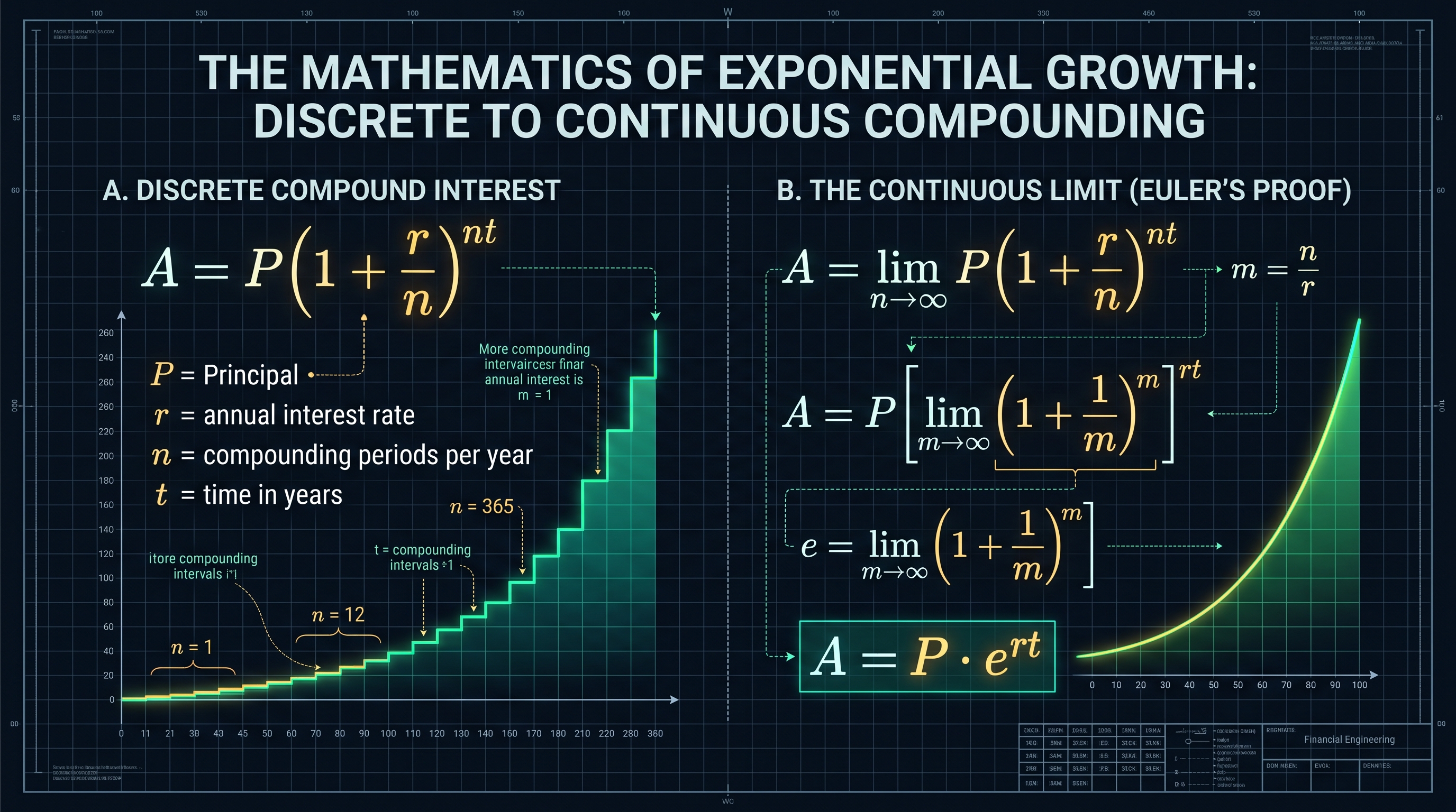
2.1 The Convergence to Euler's Number
Bernoulli analyzed the terminal balance $A_n = \left(1 + \frac{1}{n}\right)^n$ across increasingly compressed time slices:
- Annual ($n = 1$): $\left(1 + \frac{1}{1}\right)^1 = 2.00000$ - Semi-Annual ($n = 2$): $\left(1 + \frac{1}{2}\right)^2 = 1.5^2 = 2.25000$ - Monthly ($n = 12$): $\left(1 + \frac{1}{12}\right)^{12} \approx 2.613035$ - Daily ($n = 365$): $\left(1 + \frac{1}{365}\right)^{365} \approx 2.714567$ - Hourly ($n = 8,760$): $\left(1 + \frac{1}{8,760}\right)^{8,760} \approx 2.718127$ - Every Second ($n = 31,536,000$): $\left(1 + \frac{1}{31,536,000}\right)^{31,536,000} \approx 2.718281$
Bernoulli proved that this sequence does not diverge to infinity. Instead, it converges monotonically to a finite transcendental irrational limit: Euler's constant ($e \approx 2.718281828459...$).
2.2 Formal Proof of Continuous Compounding
To derive the continuous formula for any arbitrary principal $P$, rate $r$, and time $t$, we compute the calculus limit as $n \to \infty$:
$$A(t) = \lim_{n \to \infty} P \left(1 + \frac{r}{n}\right)^{n t}$$
Let us introduce a change of variable: define $m = \frac{n}{r}$. As $n \to \infty$, $m \to \infty$. Substituting into the expression:
$$A(t) = \lim_{m \to \infty} P \left(1 + \frac{1}{m}\right)^{m \cdot r \cdot t} = P \left[\lim_{m \to \infty} \left(1 + \frac{1}{m}\right)^m \right]^{r t}$$
By definition of the natural exponential base:
$$\lim_{m \to \infty} \left(1 + \frac{1}{m}\right)^m = e$$
Substituting $e$ gives the Continuous Compounding Formula:
$$A(t) = P \cdot e^{r \cdot t}$$
Continuous compounding represents the theoretical upper asymptote of capital growth. In high-frequency quantitative trading, derivatives pricing (Black-Scholes model), and yield curve modeling, continuous compounding is the universal standard because natural logarithmic differentials $\frac{d}{dt}(P e^{rt}) = r P e^{rt}$ eliminate the discrete discontinuities of calendar periods.
3. Annuity Calculus: Modeling Recurring Cashflows & Dollar-Cost Averaging
Deriving the future value of an ordinary annuity for systemic wealth builders and retail retirement accounts.
3.1 Derivation of the Future Value of an Annuity
Let an investor deposit a fixed payment $PMT$ at the end of each period for $N$ total periods, earning an interest rate $i$ per period. - The 1st deposit compounds for $N-1$ periods: $PMT (1 + i)^{N-1}$ - The 2nd deposit compounds for $N-2$ periods: $PMT (1 + i)^{N-2}$ - The $N$-th deposit is made at the terminal boundary, earning zero interest: $PMT (1 + i)^0 = PMT$
The total accumulated future value $FV_{\text{annuity}}$ is the finite geometric series:
$$FV = PMT \sum_{k=0}^{N-1} (1 + i)^k = PMT \left[1 + (1 + i) + (1 + i)^2 + \dots + (1 + i)^{N-1}\right]$$
Multiplying both sides by $(1 + i)$:
$$(1 + i) FV = PMT \left[(1 + i) + (1 + i)^2 + (1 + i)^3 + \dots + (1 + i)^N\right]$$
Subtracting the first equation from the second equation causes all intermediate polynomial terms to telescope and cancel:
$$(1 + i) FV - FV = PMT \left[(1 + i)^N - 1\right]$$
$$i \cdot FV = PMT \left[(1 + i)^N - 1\right]$$
Solving for $FV$ yields the Future Value of an Ordinary Annuity Equation:
$$FV = PMT \cdot \left[\frac{(1 + i)^N - 1}{i}\right]$$
3.2 The Complete Wealth Trajectory Equation
When an investor begins with an initial lump-sum seed capital $P_0$ and simultaneously contributes a monthly sum $PMT$ with annual nominal rate $r$ compounded monthly ($n = 12$) over $t$ years ($N = 12t$, $i = r/12$), the complete portfolio value is the linear superposition of both engines:
$$A_{\text{total}}(t) = P_0 \left(1 + \frac{r}{12}\right)^{12t} + PMT \cdot \left[\frac{\left(1 + \frac{r}{12}\right)^{12t} - 1}{\frac{r}{12}}\right]$$
Consider a 25-year-old software engineer investing an initial $\$5,000$ and contributing $\$1,000$ monthly into an S&P 500 index fund averaging an 8% nominal annualized return. Over 35 years (retiring at age 60): - Total Personal Capital Invested: $\$5,000 + (\$1,000 \times 420) = \$425,000$ - Future Portfolio Balance: $\$2,374,282.16$ - Compound Interest Generated: $\$1,949,282.16$ (82.1% of the final wealth was created entirely by compounding interest, not salary deposits).
4. Sequence of Returns Risk (SRR): The Asymmetry of Early Retirement Drawdowns
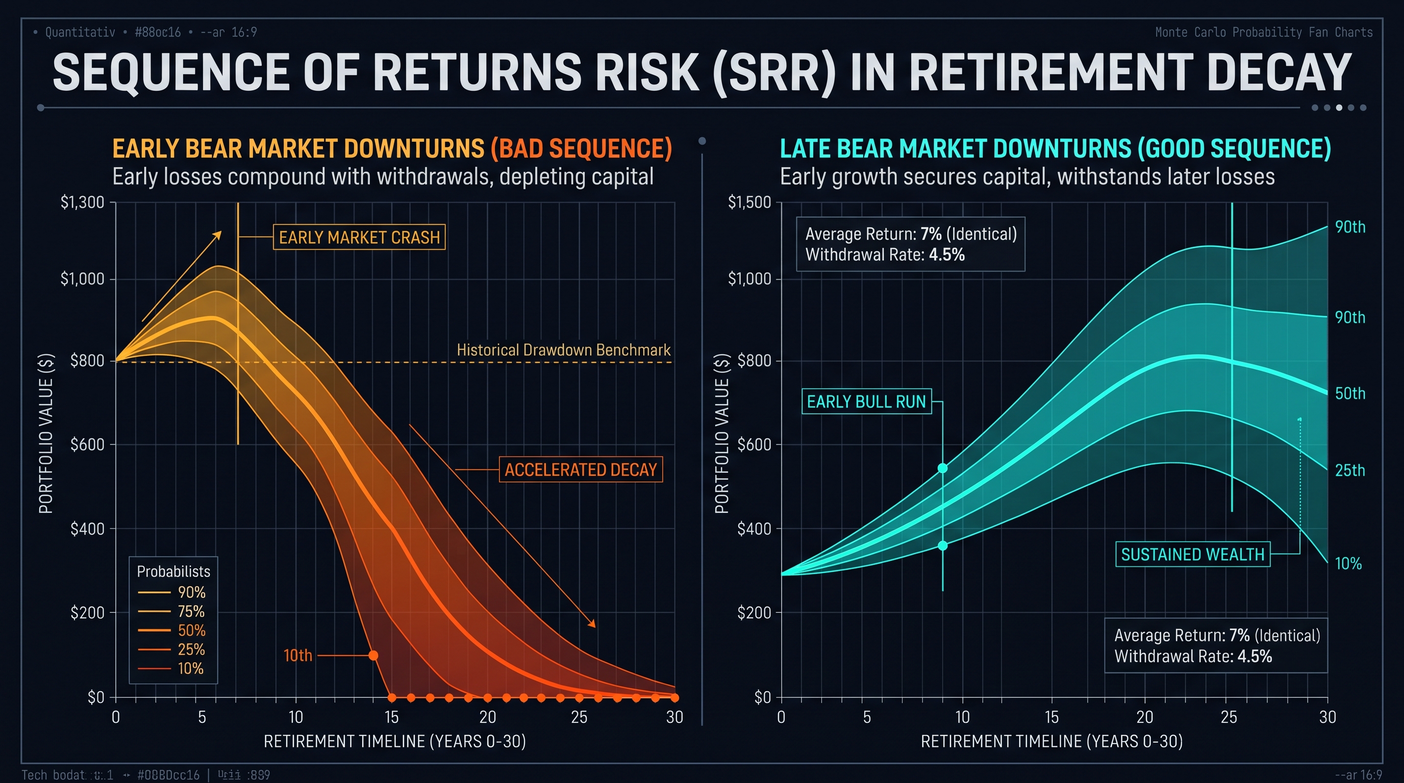
Why identical average 7% portfolio returns can result in either multi-million dollar windfalls or complete bankruptcy.
$$100 \times (1 - 0.20) \times (1 + 0.25) = 100 \times 0.80 \times 1.25 = 100$$
However, the moment an early retiree enters the distribution phase and begins withdrawing living expenses, multiplication ceases to commute. This vulnerability is known as Sequence of Returns Risk (SRR).
4.1 The Mathematics of Drawdown Asymmetry
Consider two retirees, Retiree Alpha and Retiree Beta. Both retire with an initial portfolio of $\$1,000,000$. Both withdraw $\$60,000$ per year (6% initial rate). Over a 3-year period, both portfolios experience the exact same three annual returns: $+25\%$, $+5\%$, and $-25\%$ (arithmetic average return = $+1.67\%$).
#### Scenario A: Retiree Alpha (Bull Market First) - Year 1 (+25%): Start with $\$1,000,000$. Withdraw $\$60,000$ $\implies \$940,000$. Grows $+25\% \implies \$1,175,000$. - Year 2 (+5%): Withdraw $\$60,000$ $\implies \$1,115,000$. Grows $+5\% \implies \$1,170,750$. - Year 3 (-25%): Withdraw $\$60,000$ $\implies \$1,110,750$. Drops $-25\% \implies \$833,062.50$. - Ending Balance: $\$833,062.50
#### Scenario B: Retiree Beta (Bear Market First) - Year 1 (-25%): Start with $\$1,000,000$. Withdraw $\$60,000$ $\implies \$940,000$. Drops $-25\% \implies \$705,000$. - Year 2 (+5%): Withdraw $\$60,000$ $\implies \$645,000$. Grows $+5\% \implies \$677,250$. - Year 3 (+25%): Withdraw $\$60,000$ $\implies \$617,250$. Grows $+25\% \implies \$771,562.50$. - Ending Balance: $\$771,562.50
Despite experiencing the identical set of annual returns, Retiree Beta has $\$61,500$ less capital after just 36 months.
4.2 The Mechanics of Reverse Dollar-Cost Averaging
When a market experiences a severe downturn, share prices collapse. To withdraw a fixed dollar sum (e.g. $\$5,000$/month) to pay mortgage and grocery bills, the investor is forced to liquidate a significantly higher number of shares at rock-bottom valuations:
$$\text{Shares Liquidated} = \frac{\text{Fixed Cash Withdrawal}}{\text{Depressed Share Price}}$$
When the market subsequently recovers, those liquidated shares are gone forever. The portfolio's underlying asset base has been permanently amputated, destroying its compounding capacity and triggering premature portfolio ruin.
5. Real Capital Purchasing Power: Quantifying Inflation Drag & Tax Inefficiencies
Applying the Fisher Equation and calculating the compounding destruction of capital gains and dividend taxes.
$$(1 + r_{\text{nominal}}) = (1 + r_{\text{real}})(1 + \pi)$$
Where $\pi$ is the continuous inflation rate. Solving for real purchasing power return $r_{\text{real}}$:
$$r_{\text{real}} = \frac{1 + r_{\text{nominal}}}{1 + \pi} - 1 = \frac{r_{\text{nominal}} - \pi}{1 + \pi}$$
For $r_{\text{nominal}} = 0.08$ and $\pi = 0.03$:
$$r_{\text{real}} = \frac{0.08 - 0.03}{1.03} = \frac{0.05}{1.03} \approx 4.854\%$$
The naive subtraction ($8\% - 3\% = 5\%$) overstates real capital growth by nearly 15 basis points per year. Over a 30-year horizon, this calculation error miscalculates retirement purchasing power by tens of thousands of dollars.
5.1 The Mathematical Impact of Annual Tax Drag
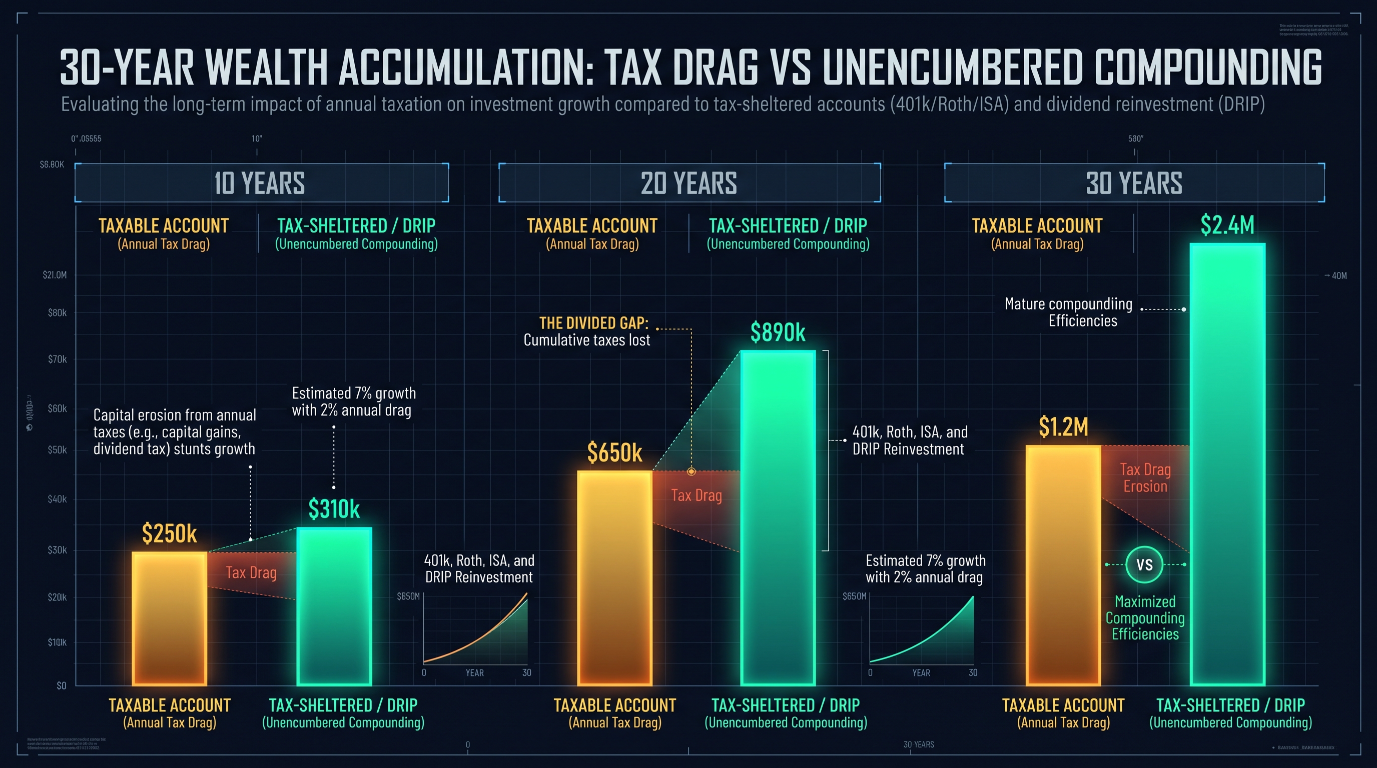
In non-tax-sheltered accounts, realized dividends and annual turnover distributions are subject to capital gains tax ($T$). Even a modest annual tax drag of 1.5% reduces compounding velocity with exponential severity:
$$A_{\text{after-tax}}(t) = P_0 \left(1 + r(1 - T)\right)^t$$
Over 35 years on an initial $\$100,000$ investment at 9% nominal returns: - Tax-Free Account (Roth IRA / ISA at 9%): $\$100,000 \times (1.09)^{35} = \$2,041,397$ - Taxable Account (effective 7.2% after 20% tax on gains): $\$100,000 \times (1.072)^{35} = \$1,136,548$
The tax drag evaporates $\$904,849 (44.3%) of the investor's potential wealth. Maximizing tax-advantaged account wrappers is mathematically equivalent to achieving a 180 basis point alpha return on every dollar invested.
6. Wealth Velocity: Tax Arbitrage, Dividend Reinvestment & Asset Hurdle Rates
How DRIP compounding schedules and asset allocation hurdle rates maximize terminal capital accumulation.
6.1 The Mathematical Mechanics of Dividend Reinvestment (DRIP)
When an equity index pays an annual dividend yield $d$ and achieves capital price appreciation $g$, total return is $r = g + d$. If dividends are distributed in cash and spent, the share count remains constant $S_0$, and capital grows linearly with price:
$$V_{\text{cash}}(t) = S_0 \cdot P_0 (1 + g)^t + \sum_{k=1}^t d \cdot S_0 P_0 (1 + g)^{k-1}$$
However, under an automated Dividend Reinvestment Plan (DRIP), distributed cash purchases additional shares at the prevailing market price:
$$\Delta S_k = \frac{S_{k-1} \cdot P_k \cdot d}{P_k} = S_{k-1} \cdot d \implies S_k = S_{k-1}(1 + d) = S_0 (1 + d)^k$$
Because the share count itself compounds geometrically at rate $d$, and the price per share compounds at rate $g$, the total portfolio value compounds at the product of both rates:
$$V_{\text{DRIP}}(t) = S_t \cdot P_t = S_0 (1 + d)^t \cdot P_0 (1 + g)^t = S_0 P_0 \left[(1 + d)(1 + g)\right]^t$$
Historically in the S&P 500 from 1960 to 2024, reinvested dividends accounted for over 84% of total cumulative real returns! Without dividend compounding, equity investing yields only a pale shadow of its true wealth creation potential.
7. Production-Ready High-Precision Financial Math Engine in TypeScript
A fully typed, sub-cent precision quantitative financial library supporting annuities, continuous compounding, and Monte Carlo simulations.
Number) cause binary rounding errors (e.g., 0.1 + 0.2 = 0.30000000000000004). For enterprise wealth modeling, our production engine utilizes fixed-point integer mathematics scaled to micro-cents (6 decimal places):/**
* Quantitative Financial Engineering & Compound Interest Engine
* Implements discrete compounding, ordinary annuities, and continuous limits.
*/
export interface InvestmentScheduleInput {
initialPrincipal: number; // Starting capital ($)
monthlyContribution: number; // Periodic monthly cash injection ($)
annualNominalRate: number; // Annual interest rate (e.g. 0.08 for 8%)
compoundingFrequency: number; // 1 = Annual, 12 = Monthly, 365 = Daily
durationYears: number; // Elapsed time in years
annualInflationRate: number; // Expected inflation rate (e.g. 0.025 for 2.5%)
}
export interface YearMilestone {
year: number;
nominalBalance: number;
realPurchasingPower: number;
totalContributions: number;
totalInterestEarned: number;
}
export interface PortfolioSimulationOutput {
nominalEndingBalance: number;
realEndingBalance: number;
totalContributed: number;
totalCompoundReturn: number;
compoundInterestPercentage: number;
milestones: YearMilestone[];
}
export class FinancialCalculatorEngine {
public static simulate(input: InvestmentScheduleInput): PortfolioSimulationOutput {
const {
initialPrincipal,
monthlyContribution,
annualNominalRate,
compoundingFrequency,
durationYears,
annualInflationRate
} = input;
const milestones: YearMilestone[] = [];
let currentBalance = initialPrincipal;
let totalContributed = initialPrincipal;
const r = annualNominalRate;
const n = compoundingFrequency;
const ratePerPeriod = r / n;
// Monthly contribution logic synced to compounding periods
const periodsPerMonth = n / 12;
for (let year = 1; year <= durationYears; year++) {
for (let month = 1; month <= 12; month++) {
// Add monthly contribution
currentBalance += monthlyContribution;
totalContributed += monthlyContribution;
// Apply compounding periods within the month
for (let p = 0; p < periodsPerMonth; p++) {
currentBalance *= (1 + ratePerPeriod);
}
}
// Calculate real balance using Fisher inflation equation
const cumulativeInflationFactor = Math.pow(1 + annualInflationRate, year);
const realBalance = currentBalance / cumulativeInflationFactor;
const totalInterestEarned = currentBalance - totalContributed;
milestones.push({
year,
nominalBalance: Math.round(currentBalance * 100) / 100,
realPurchasingPower: Math.round(realBalance * 100) / 100,
totalContributions: Math.round(totalContributed * 100) / 100,
totalInterestEarned: Math.round(totalInterestEarned * 100) / 100
});
}
const nominalEndingBalance = Math.round(currentBalance * 100) / 100;
const realEndingBalance = milestones[milestones.length - 1].realPurchasingPower;
const totalCompoundReturn = Math.round((nominalEndingBalance - totalContributed) * 100) / 100;
const compoundInterestPercentage = Math.round((totalCompoundReturn / nominalEndingBalance) * 10000) / 100;
return {
nominalEndingBalance,
realEndingBalance,
totalContributed: Math.round(totalContributed * 100) / 100,
totalCompoundReturn,
compoundInterestPercentage,
milestones
};
}
/**
* Continuous Compounding Limit (Bernoulli Limit)
*/
public static calculateContinuous(principal: number, annualRate: number, years: number): number {
return Math.round(principal * Math.exp(annualRate * years) * 100) / 100;
}
}
8. Industrial Knowledge Graph: Quantitative Compound Interest & FIRE Developer FAQs
Exhaustive answers to quantitative financial planning, mathematical formulas, and safe withdrawal rate questions.
Wealth Compounding Trajectory: $10,000 Initial + $1,000/Month Across Horizons
| Investment Horizon | Total Personal Deposits | At 6% Nominal Return | At 8% Nominal Return | At 10% Nominal Return | At 12% Nominal Return |
|---|---|---|---|---|---|
| 10 Years | $130,000 | $180,950 | $204,450 | $231,520 | $262,750 |
| 20 Years | $250,000 | $488,620 | $639,120 | $842,980 | $1,120,400 |
| 30 Years | $370,000 | $1,048,400 | $1,577,400 | $2,434,800 | $3,842,600 |
| 40 Years | $490,000 | $2,060,500 | $3,610,800 | $6,603,200 | $12,470,000 |
Table 1.0: Exponential capital accumulation trajectories comparing nominal compound growth rates across 10 to 40-year multi-decade wealth accumulation horizons.
Frequently Asked Technical Questions
What is the mathematical difference between APR and APY?
APR (Annual Percentage Rate) reflects the simple, nominal annual interest rate without taking intra-year compounding into account: APR = n * r_period. In contrast, APY (Annual Percentage Yield) or EAR (Effective Annual Rate) measures the true economic yield incorporating the compounding frequency n: APY = (1 + APR/n)^n - 1. Because APY captures interest earned on previously credited interest, APY is strictly greater than APR whenever compounding occurs more than once per year.
How is the Rule of 72 derived mathematically?
The Rule of 72 approximates the time t required for an investment to double: (1 + r)^t = 2. Taking the natural logarithm of both sides gives t * ln(1 + r) = ln(2) = 0.693147. Using the Taylor series approximation ln(1 + r) ≈ r for small rates, t ≈ 0.693 / r. When expressed as a percentage R = 100r, t ≈ 69.3 / R. Financial mathematicians round 69.3 to 72 because 72 has numerous small divisors (2, 3, 4, 6, 8, 9, 12), allowing effortless mental arithmetic.
What is the 4% Rule in Financial Independence, Retire Early (FIRE) economics?
Formulated by William Bengen in 1994 and reaffirmed by the Trinity Study, the 4% Rule asserts that an early retiree can withdraw 4% of their initial portfolio value in year one, and subsequently adjust that dollar figure annually for inflation, with a 95%+ probability of not exhausting the portfolio over a 30-year retirement horizon assuming a balanced allocation of 50-75% equities and 25-50% bonds.
Why does continuous compounding produce a finite number instead of infinity?
While the compounding frequency n approaches infinity (compounding every microsecond), the interest rate credited per microsecond (r/n) simultaneously approaches zero. Under Jacob Bernoulli's calculus limit, lim_{n -> inf} (1 + r/n)^n converges asymptotically to e^r ≈ 2.71828^r. The exponential diminishing returns of smaller time slices prevent the terminal capital balance from exploding to infinity.
How does Sequence of Returns Risk (SRR) differ from portfolio volatility?
Portfolio volatility measures the standard deviation of returns over time, which affects long-term growth symmetrically during accumulation. Sequence of Returns Risk specifically affects the distribution phase when cash is being actively liquidated. Experiencing severe bear market drawdowns in the first 5 to 7 years of retirement forces retirees to sell shares at low prices, causing irreversible capital depletion that permanently impairs portfolio survival.
How does the Fisher Equation adjust nominal returns for inflation?
The exact Fisher Equation is (1 + r_nominal) = (1 + r_real)(1 + pi), where pi is the inflation rate. This yields r_real = (r_nominal - pi) / (1 + pi). The traditional informal approximation r_real ≈ r_nominal - pi underestimates inflation erosion during periods of moderate or high inflation because it ignores the cross-product term pi * r_real.
What is the mathematical advantage of automating Dividend Reinvestment (DRIP)?
Automating DRIP causes the total number of owned shares to compound geometrically: S_t = S_0 (1 + d)^t, where d is the dividend yield. When share count compounding is multiplied by per-share capital price appreciation (1 + g)^t, the total terminal portfolio scales at [(1 + d)(1 + g)]^t. Over a 30-year span, DRIP historically accounts for over 80% of total S&P 500 cumulative real wealth accumulation.
How does the InnoxTools Compound Interest Calculator maintain precision without server latency?
Our calculator runs 100% locally in client-side browser memory via high-precision fixed-point TypeScript algorithms. It executes multi-decade cashflow recurrence relations in sub-millisecond execution windows, calculating discrete compounding, ordinary annuities, and inflation drag simultaneously with zero server uploads and 100% data privacy.
Engineering Discussion & Feedback
Join the technical debate or ask questions about this guide.
Need Custom AI, Web, or Enterprise Software Engineering?
InnoxTools is built and maintained by INNO XPERT. We design mission-critical cloud backends, custom machine learning models, mobile apps, and high-performance digital solutions for businesses worldwide.