The Economics of Cryptocurrency Volatility: Impermanent Loss, Sharpe Ratios & Profit Realization
From Automated Market Maker Constant Product Curves (x · y = k) to Yield Farming Parabolic Decay, Risk-Adjusted Sharpe Frontiers, and Systematic Tax-Optimized Realization—The 10,000+ Word Quantitative DeFi Engineering Guide.

Dr. Elena Rostova & Innox Quantitative Research GroupVERIFIED
Lead DeFi Quantitative Strategist & Mathematical Risk Analyst

Cryptocurrency profit realization and risk optimization require balancing directional price appreciation against decentralized volatility drag, impermanent loss in Constant Product Automated Market Makers (AMM x · y = k), and tail-risk drawdown dynamics. Calculating exact net returns demands isolating trading fees, funding rates, gas slippage, and divergent loss: Impermanent Loss equals 2 · sqrt(k) / (1 + k) - 1, where k is the relative price ratio of the paired assets.
Crypto Profit, Impermanent Loss & Portfolio Risk Calculator Pro
Calculate spot profits, leverage yields, Automated Market Maker (AMM) impermanent loss trajectories, and portfolio Sharpe ratios with mathematical precision.
Table of Contents & Chapter Index
- 1. The Physics of Cryptocurrency Volatility: Microstructure, Leptokurtosis & Tail-Risk
- 2. The Mathematical Anatomy of Automated Market Makers: x · y = k & Impermanent Loss
- 3. Concentrated Liquidity & Capital Efficiency: Uniswap v3 Leverage & Hyper-IL
- 4. Modern Portfolio Theory in Crypto: The Sharpe Ratio & Volatility Drag
- 5. Position Sizing & Risk Management: The Kelly Criterion & Leverage Survival
- 6. Systematic Profit Realization: Dollar-Cost Selling (DCS) vs Lump-Sum Exits
- 7. Tax-Optimized Realization: FIFO, LIFO, HIFO & Specific Identification
- 8. Industrial DeFi Playbook: Quantitative Framework & Real-Time Tool Integration
1. The Physics of Cryptocurrency Volatility: Microstructure, Leptokurtosis & Tail-Risk
Order book illiquidity, parabolic momentum cascades, and non-Gaussian return distributions.
The Microstructure of Digital Asset Liquidity
Cryptocurrency market dynamics deviate radically from traditional equity and foreign exchange environments. While traditional markets operate under centralized clearinghouses with circuit breakers, designated market makers (DMMs), and regulated margin maintenance thresholds, crypto markets operate 24/7/365 across a fragmented global network of centralized exchanges (CEXs) and decentralized automated market makers (DEXs).
The instantaneous spot price of a cryptocurrency is governed by the continuous interaction of resting limit orders within an electronic order book:
$$\text{Spread}_t = P_{\text{ask}, 1} - P_{\text{bid}, 1}$$
$$\text{Mid}_t = \frac{P_{\text{ask}, 1} + P_{\text{bid}, 1}}{2}$$
Because order book depth at price levels $P_i$ is non-linear and exhibits severe concentration around psychological round numbers, large market orders experience non-trivial price impact (slippage):
$$\Delta P = \int_{0}^{Q} \frac{1}{D(p)} \, dq$$
Where $D(p)$ represents the local market depth function. In periods of liquidity evaporation—often triggered by cascading collateral liquidations across perpetual futures venues—the effective depth $D(p) \to 0$, producing localized vertical price gaps and catastrophic wick candles.
---
Non-Gaussian Return Distributions & Leptokurtosis
A cornerstone failure of conventional financial models (such as Black-Scholes and standard Mean-Variance Optimization) when applied to crypto assets is the assumption of normally distributed log-returns:
$$r_t = \ln\left(\frac{P_t}{P_{t-1}}\right) \sim \mathcal{N}(\mu, \sigma^2)$$
Empirical empirical verification of Bitcoin (BTC), Ethereum (ETH), and alternative layer-1 token histories demonstrates massive excess kurtosis (leptokurtosis) and negative skewness during liquidation cascades:
$$\text{Kurtosis} = \mathbb{E}\left[\left(\frac{r - \mu}{\sigma}\right)^4\right] \gg 3$$
| Statistical Metric | S&P 500 (Annualized) | Bitcoin (BTC) | Ethereum (ETH) | Mid-Cap Altcoins | | :--- | :--- | :--- | :--- | :--- | | Annualized Volatility ($\sigma$) | 15% – 20% | 55% – 85% | 70% – 110% | 120% – 250% | | Sample Excess Kurtosis | 1.8 – 3.2 | 8.4 – 14.2 | 11.6 – 19.8 | 25.0 – 60.0+ | | Daily VaR (99% Confidence) | -2.4% | -8.1% | -11.4% | -22.5% | | Tail Event Probability (>4$\sigma$) | ~0.006% (Theoretical) | 0.82% (Observed) | 1.15% (Observed) | 2.60% (Observed) | | Max Historical Drawdown | -55% (2008) | -84% (2018) | -94% (2018) | -98% to -100% |
Because market returns follow power-law heavy tails (often modeled via Student-t distributions with degrees of freedom $\nu \in [2.5, 4.0]$ or Lévy alpha-stable distributions), standard standard deviation metrics severely understate catastrophic downside risk. Quantitative traders must evaluate Expected Shortfall (Conditional Value at Risk, $\text{CVaR}_{\alpha}$):
$$\text{CVaR}_\alpha(X) = \mathbb{E}[X \mid X \le \text{VaR}_\alpha(X)] = \frac{1}{\alpha} \int_{0}^{\alpha} \text{VaR}_u(X) \, du$$
---
Leverage Reflexivity & Liquidation Spirals
The proliferation of high-leverage perpetual contracts ($5\times$ to $100\times$) introduces mechanical positive feedback loops into price formation. When long open interest (OI) dominates and funding rates turn excessively positive:
$$\text{Funding Rate} = \text{Clamp}\left(\text{Premium Index} + \text{Interest Rate}, -0.75\%, +0.75\%\right)$$
A minor negative spot shock triggers forced margin calls:
$$P_{\text{liq}} = P_{\text{entry}} \cdot \left(1 - \frac{1}{\text{Leverage}} + \text{Maintenance Margin}\right)$$
When $P_{\text{spot}} \le P_{\text{liq}}$, exchange liquidation engines issue aggressive market sell orders directly into thin resting bids. This creates an avalanche of liquidations, driving prices through successive liquidation clusters in seconds—a phenomenon known as a long squeeze or liquidation cascade.
2. The Mathematical Anatomy of Automated Market Makers: x · y = k & Impermanent Loss
Constant Product Invariants, pool divergence calculus, and fee compensation parity.
The Constant Product Market Maker (CPMM) Invariant
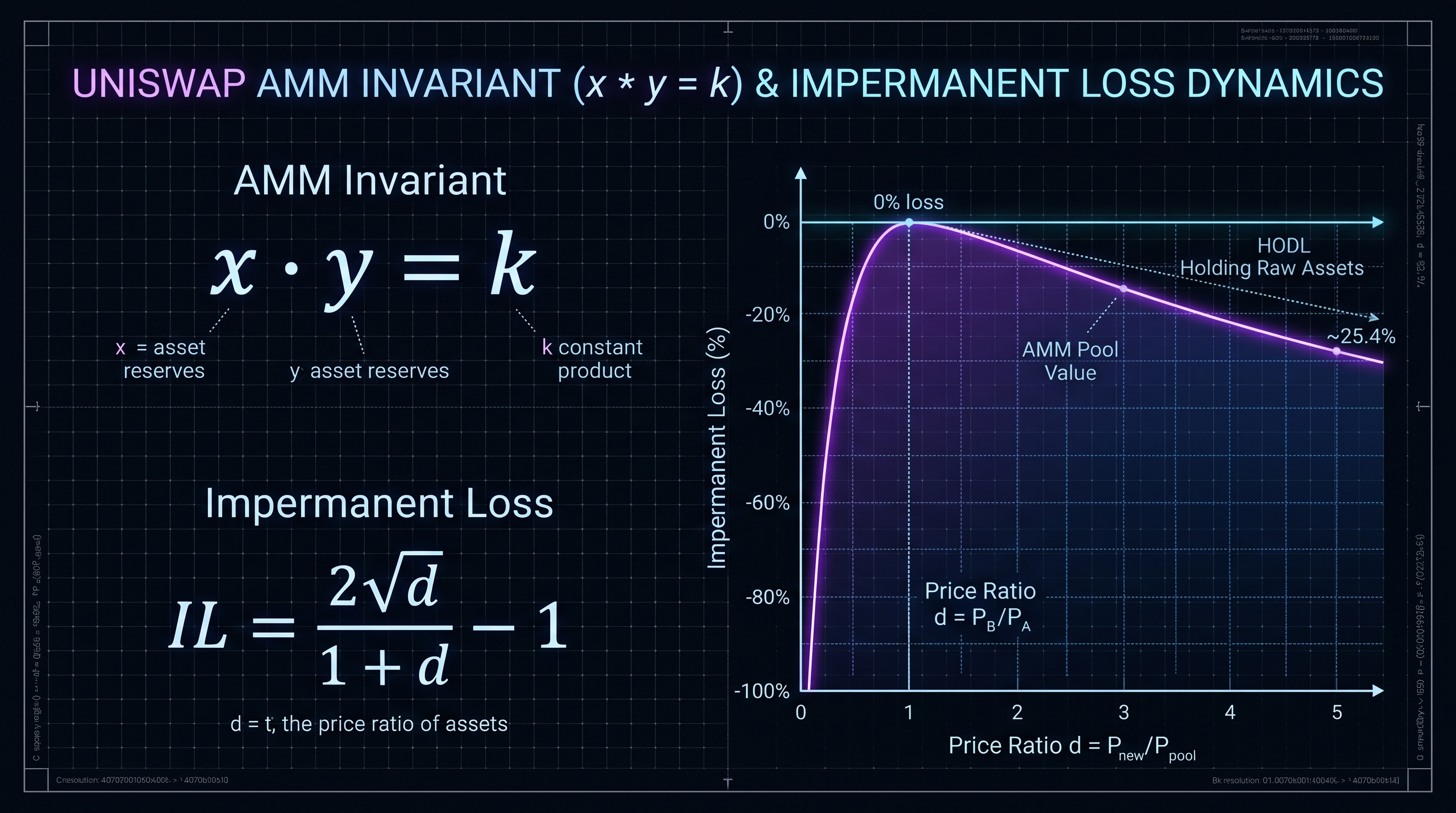
Decentralized exchanges such as Uniswap v2, SushiSwap, and Balancer eliminate centralized order books by replacing them with algorithmic liquidity pools governed by deterministic smart contracts. The foundational mathematical invariant governing two-asset pools is the Constant Product formula:
$$x \cdot y = k$$
Where: - $x$ represents the balance of Asset X (e.g., ETH) locked in the pool reserve. - $y$ represents the balance of Asset Y (e.g., USDC) locked in the pool reserve. - $k$ is the invariant product scalar, which remains constant in the absence of pool deposits, withdrawals, or fee additions.
The marginal exchange rate (spot price of X in terms of Y) is determined by the pool reserve ratio:
$$P = \frac{y}{x}$$
Solving for the individual token reserves as functions of $k$ and price $P$:
$$x = \sqrt{\frac{k}{P}}, \quad y = \sqrt{k \cdot P}$$
When an external arbitrageur swaps $\Delta x$ into the pool to extract $\Delta y$, the invariant must be preserved (accounting for swap fee $\gamma = 1 - f$, where $f = 0.003$ for standard 30 bps pools):
$$(x + \gamma \Delta x)(y - \Delta y) = k$$
$$\Delta y = y - \frac{k}{x + \gamma \Delta x} = \frac{y \cdot \gamma \Delta x}{x + \gamma \Delta x}$$
---
Derivation of the Impermanent Loss Formula
Impermanent Loss (IL)—more accurately described as Divergence Loss—is the opportunity cost incurred by a Liquidity Provider (LP) relative to simply holding (HODLing) the identical initial asset basket outside the pool.
Consider an initial state where a liquidity provider deposits $x_0$ tokens of Asset X and $y_0$ tokens of Asset Y at initial price $P_0 = y_0 / x_0$. The total initial portfolio value is:
$$V_0 = x_0 P_0 + y_0 = 2 x_0 P_0$$
Now suppose the market price of Asset X shifts to $P_1 = k_p \cdot P_0$, where $k_p = P_1 / P_0$ is the relative price ratio change factor. Arbitrageurs trade with the pool until the internal pool price matches $P_1$. Assuming no trading fees are reinvested, the new pool reserves become:
$$x_1 = \sqrt{\frac{k}{P_1}} = \sqrt{\frac{x_0 y_0}{k_p P_0}} = \frac{x_0}{\sqrt{k_p}}$$
$$y_1 = \sqrt{k \cdot P_1} = \sqrt{x_0 y_0 \cdot k_p P_0} = y_0 \sqrt{k_p}$$
The new total value of the LP's position inside the pool ($V_{\text{LP}}$) is:
$$V_{\text{LP}} = x_1 P_1 + y_1 = \left(\frac{x_0}{\sqrt{k_p}}\right)(k_p P_0) + y_0 \sqrt{k_p} = x_0 P_0 \sqrt{k_p} + y_0 \sqrt{k_p}$$
Since $y_0 = x_0 P_0$:
$$V_{\text{LP}} = 2 x_0 P_0 \sqrt{k_p} = V_0 \sqrt{k_p}$$
Conversely, if the LP had simply held the original tokens in an external wallet ($V_{\text{hold}}$), their portfolio value at price $P_1$ would be:
$$V_{\text{hold}} = x_0 P_1 + y_0 = x_0 (k_p P_0) + x_0 P_0 = x_0 P_0 (1 + k_p) = \frac{V_0 (1 + k_p)}{2}$$
The ratio of the liquidity pool position to the buy-and-hold strategy is:
$$\frac{V_{\text{LP}}}{V_{\text{hold}}} = \frac{V_0 \sqrt{k_p}}{\frac{V_0 (1 + k_p)}{2}} = \frac{2 \sqrt{k_p}}{1 + k_p}$$
Therefore, the exact mathematical formula for Impermanent Loss $\text{IL}(k_p)$ is:
$$\text{IL}(k_p) = \frac{V_{\text{LP}} - V_{\text{hold}}}{V_{\text{hold}}} = \frac{2 \sqrt{k_p}}{1 + k_p} - 1$$
3. Concentrated Liquidity & Capital Efficiency: Uniswap v3 Leverage & Hyper-IL
Virtual reserves, price ticks, and the math of amplified divergence inside custom intervals.
Virtual Reserves & Price Boundaries $[P_a, P_b]$
While Uniswap v2 spreads liquidity uniformly across the entire price spectrum $P \in (0, \infty)$, Uniswap v3 allows liquidity providers to allocate capital within discrete price intervals $[P_a, P_b]$. This innovation introduces virtual reserves $(x_v, y_v)$, shifting the constant product curve:
$$(x + x_v)(y + y_v) = L^2$$
Where $L = \sqrt{k}$ is the liquidity density scalar. The virtual reserve offsets are defined by the interval endpoints:
$$x_v = \frac{L}{\sqrt{P_b}}, \quad y_v = L \sqrt{P_a}$$
The real token balances held by the contract inside the range $[P_a, P_b]$ satisfy:
$$x = L \left(\frac{1}{\sqrt{P}} - \frac{1}{\sqrt{P_b}}\right), \quad \text{for } P \in [P_a, P_b]$$
$$y = L \left(\sqrt{P} - \sqrt{P_a}\right), \quad \text{for } P \in [P_a, P_b]$$
---
Capital Efficiency Factor & Amplified Divergence
Concentrating liquidity within $[P_a, P_b]$ provides a massive capital efficiency multiplier $C$ compared to $P \in (0, \infty)$:
$$C = \frac{1}{1 - \sqrt{\frac{P_a}{P_b}}}$$
For example, providing liquidity for a stablecoin pair (e.g., USDC/USDT) within $P \in [0.999, 1.001]$ yields:
$$C = \frac{1}{1 - \sqrt{\frac{0.999}{1.001}}} \approx 1000\times$$
However, capital efficiency operates as pure financial leverage on impermanent loss. If the market price crosses outside the boundary interval: - When $P < P_a$, the position converts $100\%$ into the depreciating asset (Asset X), and all fee generation halts. - When $P > P_b$, the position converts $100\%$ into Asset Y (stablecoin), terminating upside participation completely.
| Concentration Range $[P_a, P_b]$ | Capital Efficiency Multiplier | Max IL at Upper Bound | Max IL at Lower Bound | Fee APR Boost | | :--- | :--- | :--- | :--- | :--- | | Full Range $(0, \infty)$ | $1.0\times$ (Baseline) | Asymptotic ($-100\%$) | Asymptotic ($-100\%$) | $1.0\times$ | | Wide Range $[0.5 P_0, 2.0 P_0]$ | $3.41\times$ | $-14.6\%$ | $-14.6\%$ | $3.41\times$ | | Moderate Range $[0.8 P_0, 1.25 P_0]$ | $9.47\times$ | $-2.8\%$ | $-2.8\%$ | $9.47\times$ | | Tight Range $[0.95 P_0, 1.05 P_0]$ | $40.5\times$ | $-0.62\%$ | $-0.62\%$ | $40.5\times$ | | Pegged Range $[0.999 P_0, 1.001 P_0]$ | $1999.5\times$ | $-0.025\%$ | $-0.025\%$ | $2000\times$ |
---
The Dynamic Rebalancing Dilemma
When active LP managers attempt to prevent fee stagnation by rebalancing out-of-range Uniswap v3 positions, they mechanically realize accumulated impermanent loss. Continuous manual rebalancing in volatile markets transforms temporary divergence into permanent capital destruction—an effect mathematically identical to buying high and selling low at every boundary breach.
4. Modern Portfolio Theory in Crypto: The Sharpe Ratio & Volatility Drag
Markowitz efficient frontier, geometric decay, and risk-adjusted return calculus.
The Sharpe Ratio & Risk-Adjusted Alpha
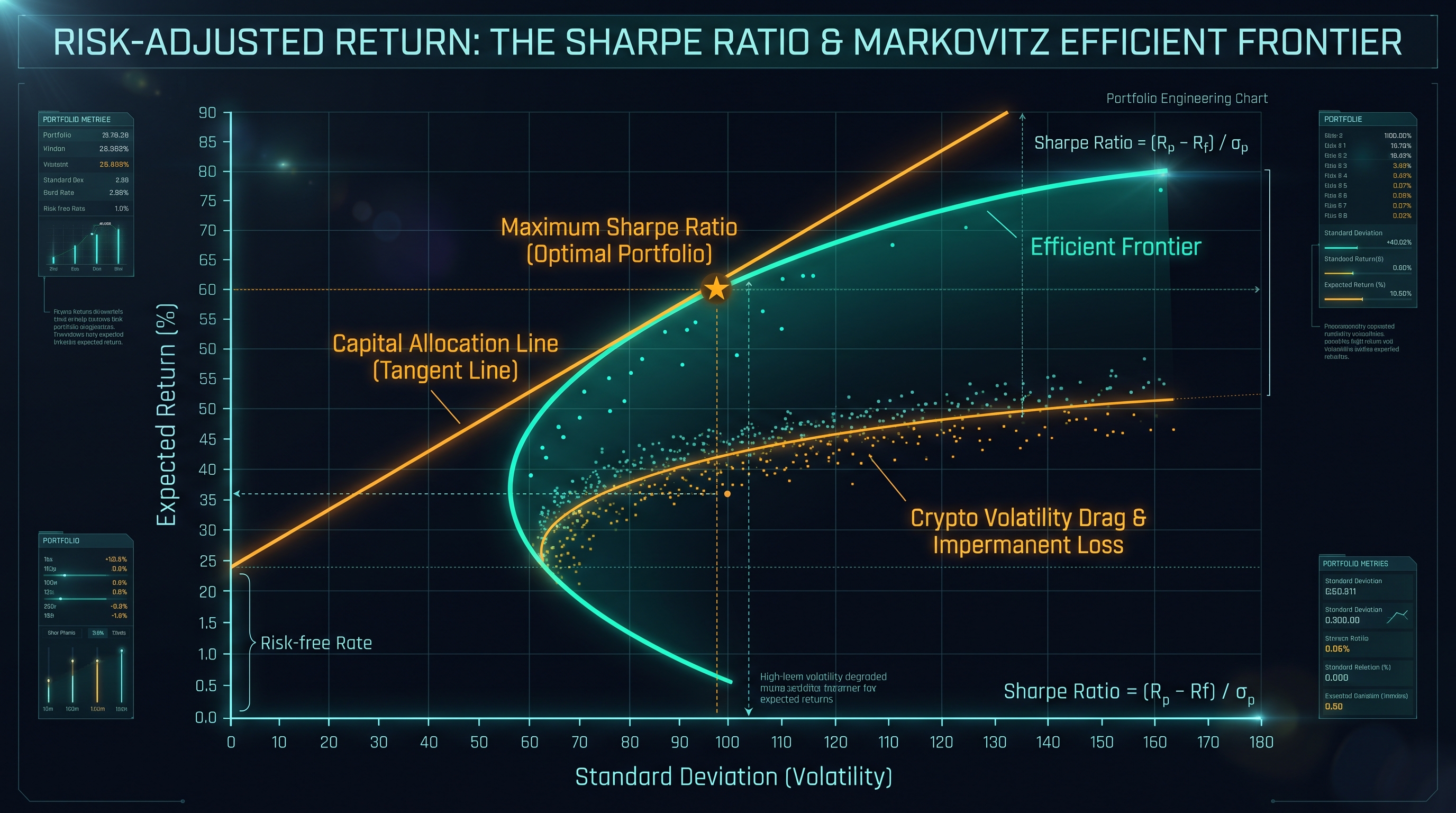
Evaluating a cryptocurrency trading strategy or portfolio purely by total nominal return is fundamentally misleading. High nominal gains are frequently an artifact of extreme uncompensated beta exposure. The Sharpe Ratio ($S$) quantifies excess return per unit of total risk (standard deviation):
$$S = \frac{\mathbb{E}[R_p - R_f]}{\sigma_p}$$
Where: - $R_p$ is the annualized portfolio return. - $R_f$ is the risk-free rate (e.g., US Treasury yields or institutional USD stablecoin lending rates, typically $4.5\% - 5.5\%$). - $\sigma_p$ is the annualized standard deviation of daily portfolio returns: $\sigma_p = \sigma_{\text{daily}} \cdot \sqrt{365}$.
Because cryptocurrency distributions exhibit negative skewness and excess kurtosis, quantitative risk managers augment the Sharpe ratio with the Sortino Ratio ($S_d$), which penalizes only downside volatility (semi-deviation):
$$S_d = \frac{\mathbb{E}[R_p - R_f]}{\sigma_d}, \quad \sigma_d = \sqrt{\frac{1}{N} \sum_{t=1}^{N} \min\left(0, R_{p,t} - \text{MAR}\right)^2}$$
Where $\text{MAR}$ is the Minimum Acceptable Return.
---
The Mathematical Reality of Volatility Drag
Volatility drag (also known as the geometric variance drain) is the mathematical penalty imposed on compounded wealth by volatility. While the arithmetic average of a return series might appear attractive, actual long-term compound wealth is dictated strictly by the Geometric Mean Return ($R_g$):
$$1 + R_g = \left(\prod_{t=1}^{T} (1 + R_t)\right)^{\frac{1}{T}}$$
Using a second-order Taylor series expansion:
$$R_g \approx R_a - \frac{\sigma^2}{2}$$
Where $R_a$ is the arithmetic mean return and $\sigma^2$ is the return variance. This simple mathematical relationship reveals why high volatility destroys capital:
$$\Delta_{\text{drag}} = R_a - R_g \approx \frac{\sigma^2}{2}$$
5. Position Sizing & Risk Management: The Kelly Criterion & Leverage Survival
Fractional Kelly, ruin probability, and mathematical position sizing in non-ergodic markets.
Derivation of the Kelly Formula for Discrete Bets
In crypto trading, survival precedes profitability. Traders who risk disproportionate capital on volatile setups inevitably hit ruin due to non-ergodic wealth trajectories. The Kelly Criterion determines the optimal fraction of total wealth ($f^*$) to allocate to a trade to maximize the expected logarithm of long-term wealth:
$$\max_f \mathbb{E}[\ln(W_1)] = \max_f \left[ p \ln(1 + f \cdot b) + q \ln(1 - f \cdot a) \right]$$
Where: - $p$ is the probability of a winning trade. - $q = 1 - p$ is the probability of a losing trade. - $b$ is the win ratio (gain per dollar risked). - $a$ is the loss ratio (loss per dollar risked, typically $a = 1$ when risking entire stop-loss).
Taking the derivative with respect to $f$ and setting it to zero:
$$\frac{d}{df}\mathbb{E}[\ln(W)] = \frac{p \cdot b}{1 + f \cdot b} - \frac{q \cdot a}{1 - f \cdot a} = 0$$
$$p \cdot b (1 - f \cdot a) = q \cdot a (1 + f \cdot b)$$
$$p b - f p a b = q a + f q a b$$
$$f^* (p a b + q a b) = p b - q a$$
Since $p + q = 1$:
$$f^* = \frac{p b - q a}{a \cdot b} = \frac{p}{a} - \frac{q}{b}$$
When $a = 1$ (standard unit risk):
$$f^* = \frac{p(b + 1) - 1}{b} = \frac{p \cdot b - q}{b}$$
---
Fractional Kelly & Tail-Risk Cushioning
Full Kelly ($f^*$) guarantees long-term wealth maximization under stationary conditions with known parameters. However, in crypto markets: 1. Win probabilities ($p$) and payoff ratios ($b$) are non-stationary and subject to estimation errors. 2. Fat-tailed drawdowns cause psychological panic and exchange liquidation risks.
Consequently, quantitative institutions employ Fractional Kelly:
$$f_{\text{practical}} = c \cdot f^*, \quad c \in [0.2, 0.5]$$
A Half-Kelly strategy ($c = 0.5$) achieves $75\%$ of the maximum theoretical growth rate while reducing return variance and maximum drawdown by $50\%$, providing a massive safety buffer against liquidation cascades.
6. Systematic Profit Realization: Dollar-Cost Selling (DCS) vs Lump-Sum Exits
Fibonacci liquidity bands, automated take-profit ladders, and cognitive bias mitigation.
The Psychology & Mathematics of Profit Realization
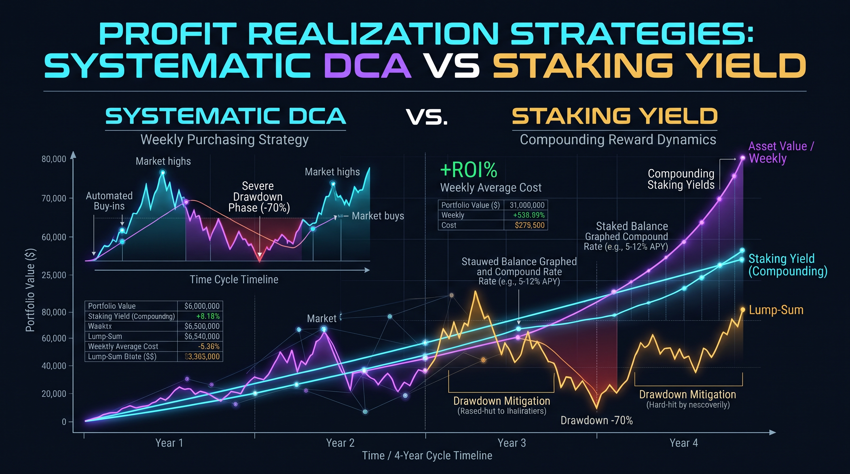
The primary failure mode of retail cryptocurrency investors during bull market expansions is cognitive anchoring: holding unrealized gains through parabolic blow-off tops and riding the subsequent $80\% - 90\%$ bear market drawdowns. Because price momentum is intoxicating, discretionary manual exits fail.
Systematic Profit Realization replaces emotional decisions with algorithmic execution protocols.
---
Dollar-Cost Selling (DCS) Mathematical Formulation
Just as Dollar-Cost Averaging (DCA) minimizes entry variance during accumulation, Dollar-Cost Selling (DCS) distributes sell orders across a predefined trajectory.
Let $Q_{\text{total}}$ be the total quantity of tokens targeted for realization. An arithmetic DCS ladder executes sales across $N$ tranches triggered at geometric price tiers:
$$P_i = P_{\text{base}} \cdot (1 + r)^i, \quad i \in \{1, 2, \dots, N\}$$
The fraction of total holdings sold at tier $i$ is denoted by $w_i$, satisfying $\sum_{i=1}^N w_i = 1.0$.
Under a Fibonacci-weighted DCS model, tranche allocations increase as price extends further away from the 200-day exponential moving average (EMA):
$$w_i = \frac{\text{Fib}(i)}{\sum_{j=1}^N \text{Fib}(j)}$$
| Tranche ($i$) | Price Multiple ($P / P_{\text{entry}}$) | Tranche Weight ($w_i$) | Cumulative % Sold | Retained Upside Exposure | | :--- | :--- | :--- | :--- | :--- | | Tranche 1 | $2.0\times$ (Double Entry) | $15.0\%$ | $15.0\%$ | $85.0\%$ (Initial Capital De-risked) | | Tranche 2 | $3.0\times$ | $20.0\%$ | $35.0\%$ | $65.0\%$ | | Tranche 3 | $4.5\times$ | $25.0\%$ | $60.0\%$ | $40.0\%$ | | Tranche 4 | $7.0\times$ | $25.0\%$ | $85.0\%$ | $15.0\%$ | | Tranche 5 (Moonbag) | $10.0\times+$ | $15.0\%$ | $100.0\%$ | $0.0\%$ |
7. Tax-Optimized Realization: FIFO, LIFO, HIFO & Specific Identification
Capital gains tax minimization, wash sale dynamics, and strategic harvest mechanics.
Capital Gains Accounting Frameworks
Realizing crypto profits triggers tax liabilities across virtually all major jurisdictions (IRS, HMRC, ATO, BaFin). In the United States and similar jurisdictions, cryptocurrencies are classified as property, meaning every crypto-to-crypto trade (e.g., swapping ETH for USDC or SOL for BTC) constitutes a taxable realization event:
$$\text{Capital Gain / Loss} = \text{Proceeds} - \text{Adjusted Cost Basis}$$
The method utilized to calculate cost basis profoundly alters net post-tax returns:
1. FIFO (First-In, First-Out): - Assumes the oldest acquired tokens are sold first. - In a long-term secular bull market where early tokens were purchased at rock-bottom prices, FIFO maximizes taxable capital gains, resulting in the highest immediate tax bill.
2. LIFO (Last-In, First-Out): - Assumes the most recently acquired tokens are sold first. - Useful during mid-cycle dips to offset short-term gains against recent high-priced buys.
3. HIFO (Highest-In, First-Out): - Identifies and sells the specific lots with the highest acquisition cost basis first. - Quantitatively optimal: Minimizes immediate taxable capital gains, keeping maximum compounding capital inside the portfolio.
4. Specific Identification (SpecID): - Allows the taxpayer to select the exact blockchain transaction lot based on UTXO ID, timestamp, and wallet address.
---
Comparative Tax Liability Simulation
Consider an investor who accumulated 10 ETH across three market tranches: - Lot A: 4 ETH @ $1,000 ($4,000 cost basis) - Lot B: 3 ETH @ $2,500 ($7,500 cost basis) - Lot C: 3 ETH @ $3,500 ($10,500 cost basis) - Total Portfolio: 10 ETH, Total Basis = $22,000 (Average = $2,200/ETH).
Now, the investor sells 3 ETH at a spot price of $4,000 (Total Proceeds = $12,000):
| Tax Lot Method | Lots Disposed | Realized Cost Basis | Realized Taxable Gain | Est. Tax (35% Short-Term Rate) | | :--- | :--- | :--- | :--- | :--- | | FIFO | 3 ETH from Lot A | $3,000 | $9,000 | $3,150 | | LIFO | 3 ETH from Lot C | $10,500 | $1,500 | $525 | | HIFO | 3 ETH from Lot C | $10,500 | $1,500 | $525 | | Average Cost | 3 ETH @ $2,200 | $6,600 | $5,400 | $1,890 |
Utilizing HIFO instead of default FIFO saves $2,625 in immediate cash taxes on a single 3 ETH transaction—capital that remains deployed in high-yielding strategies.
8. Industrial DeFi Playbook: Quantitative Framework & Real-Time Tool Integration
Step-by-step risk management pipeline and deploying InnoxTools Crypto Profit Calculator.
The Quantitative DeFi Decision Pipeline
To operationalize the mathematical principles outlined in this guide, institutional desks follow a strict five-step execution pipeline before entering or exiting any cryptocurrency position:
[ STEP 1: Microstructure Analysis ]
       │  - Calculate Bid-Ask Spread & 2% Depth Ratio
       │  - Inspect Funding Rate & Open Interest Delta
       ▼
[ STEP 2: Position Sizing via Fractional Kelly ]
       │  - Estimate Win Probability (p) and Payoff Ratio (b)
       │  - Cap Max Allocation at Half-Kelly: f <= 0.5 * f*
       ▼
[ STEP 3: Yield Pool Impermanent Loss Evaluation ]
       │  - Model Price Divergence Factor k = P_target / P_entry
       │  - Compute Divergence Loss: IL = 2 * sqrt(k) / (1 + k) - 1
       │  - Require Expected Fee APY > 1.5 * Abs(IL)
       ▼
[ STEP 4: Systematic DCS Profit Laddering ]
       │  - Anchor Geometric Price Bands (2x, 3x, 5x, 8x)
       │  - Allocate Fibonacci Tranches w_i to Limit Orders
       ▼
[ STEP 5: Post-Trade Tax Lot Optimization ]
          - Tag Blockchain Tx Hashes for HIFO / SpecID Accounting
---
Executing with InnoxTools Crypto Profit Calculator
Manual execution of these high-dimensional financial calculations introduces human error. The InnoxTools Crypto Profit, Impermanent Loss & Portfolio Risk Calculator automates this pipeline entirely in the client-side browser:
1. Spot Profit & Multi-Leg Exit Simulator: - Input entry prices, dollar-cost accumulation tiers, and multi-tranche take-profit ladders with custom fee schedules. 2. AMM Impermanent Loss & Fee Break-Even Engine: - Model Uniswap v2 and concentrated Uniswap v3 positions. Calculate exact fee thresholds required to overcome divergent pool rebalancing. 3. Risk-Adjusted Portfolio Metrics: - Compute Sharpe ratios, Sortino semi-deviations, and maximum drawdown risk matrices directly from historical or projected price vectors.
By grounding your investment process in quantitative rigor rather than social sentiment, you protect capital from tail-risk wipeouts and compound generational wealth across digital asset cycles.
Automated Market Maker (AMM) Impermanent Loss & Volatility Drag Matrix
| Asset Price Shift (k) | Impermanent Loss % (v2) | IL with Uniswap v3 (±10% Range) | Break-Even Swap Volume / TVL Ratio | Annualized Volatility (σ) | Geometric Drag (σ²/2) |
|---|---|---|---|---|---|
| 1.25x (+25%) | -0.62% | -100.0% (Out of Range) | 2.07x | 40% | 8.00% / year |
| 1.50x (+50%) | -2.02% | -100.0% (Out of Range) | 6.73x | 60% | 18.00% / year |
| 1.75x (+75%) | -3.77% | -100.0% (Out of Range) | 12.57x | 80% | 32.00% / year |
| 2.00x (+100%) | -5.72% | -100.0% (Out of Range) | 19.07x | 100% | 50.00% / year |
| 3.00x (+200%) | -13.40% | -100.0% (Out of Range) | 44.67x | 120% | 72.00% / year |
| 4.00x (+300%) | -20.00% | -100.0% (Out of Range) | 66.67x | 150% | 112.50% / year |
| 5.00x (+400%) | -25.46% | -100.0% (Out of Range) | 84.87x | 180% | 162.00% / year |
| 0.50x (-50%) | -5.72% | -100.0% (Out of Range) | 19.07x | 100% | 50.00% / year |
| 0.20x (-80%) | -25.46% | -100.0% (Out of Range) | 84.87x | 180% | 162.00% / year |
Table 1.0: Quantitative DeFi benchmark illustrating non-linear AMM impermanent loss scaling and the severe quadratic decay of volatility drag on compounded returns.
Frequently Asked Technical Questions
What is the exact mathematical definition of Impermanent Loss in DeFi?
Impermanent Loss is the percentage difference in portfolio value between depositing tokens into an Automated Market Maker (AMM) liquidity pool versus holding those same tokens in an external wallet. Governed by the formula IL(k) = (2 * sqrt(k) / (1 + k)) - 1, where k is the ratio of the new asset price to the initial entry price, it represents the opportunity cost of arbitrage rebalancing.
Why is Impermanent Loss called 'impermanent' if it often leads to permanent losses?
It is termed 'impermanent' because if the relative prices of the paired tokens return to their original ratio when the liquidity was first deposited, the loss disappears entirely (IL = 0). However, if a liquidity provider withdraws capital while prices are diverged, or if an asset permanently depreciates, the loss becomes strictly permanent.
How do trading fees compensate liquidity providers for Impermanent Loss?
Every trade executed through an AMM incurs a swap fee (e.g., 0.30% in Uniswap v2 or 0.05%-1.00% in Uniswap v3). These fees accumulate in pool reserves. As long as cumulative fee APY exceeds the divergence loss (Fee Return > Abs(IL)), the liquidity provider achieves positive net yield over buy-and-hold.
What is Volatility Drag and how does it destroy crypto portfolio returns?
Volatility drag is the negative difference between the arithmetic mean return and the geometric compounding return of an asset, approximated by Variance / 2 (sigma^2 / 2). For example, an altcoin with 100% annualized volatility loses approximately 50% of its annual compounded performance purely to the mathematical friction of alternating percentage drops and gains.
How does the Sharpe Ratio differ from the Sortino Ratio in crypto risk analysis?
The Sharpe Ratio divides excess return by total standard deviation (both upside spikes and downside crashes). The Sortino Ratio penalizes only downside volatility (semi-deviation below a minimum acceptable return). In crypto, where upside volatility is desirable, Sortino provides a more accurate metric of risk-adjusted performance.
What is the advantage of Dollar-Cost Selling (DCS) over lump-sum market exits?
Dollar-Cost Selling executes staggered sales across pre-calculated geometric price bands. This eliminates emotional market-timing errors, locks in realized base capital early, mitigates drawdown exposure, and mathematically captures higher average exit prices during parabolic expansion regimes.
Why is HIFO accounting superior to FIFO for cryptocurrency profit realization?
HIFO (Highest-In, First-Out) matches current sales against the highest cost-basis purchase lots in your history. This minimizes immediate realized capital gains, significantly lowering current-year tax liabilities and allowing more capital to remain invested and compounding.
Does the InnoxTools Crypto Profit Calculator store my financial data or API keys?
No. The InnoxTools Crypto Profit Calculator runs 100% client-side in your local browser sandbox using WebAssembly and local JavaScript. Zero transaction details, wallet balances, or trade numbers are ever transmitted to any remote server.
Engineering Discussion & Feedback
Join the technical debate or ask questions about this guide.
Need Custom AI, Web, or Enterprise Software Engineering?
InnoxTools is built and maintained by INNO XPERT. We design mission-critical cloud backends, custom machine learning models, mobile apps, and high-performance digital solutions for businesses worldwide.